
271 lines
12 KiB
Markdown
271 lines
12 KiB
Markdown
|
|
> Name
|
|
|
|
多时间框架自适应追踪止损策略Multi-timeframe-Adaptive-Tracking-Stop-Loss-Strategy
|
|
|
|
> Author
|
|
|
|
ChaoZhang
|
|
|
|
> Strategy Description
|
|
|
|
|
|
[trans]
|
|
|
|
|
|
## 概述
|
|
|
|
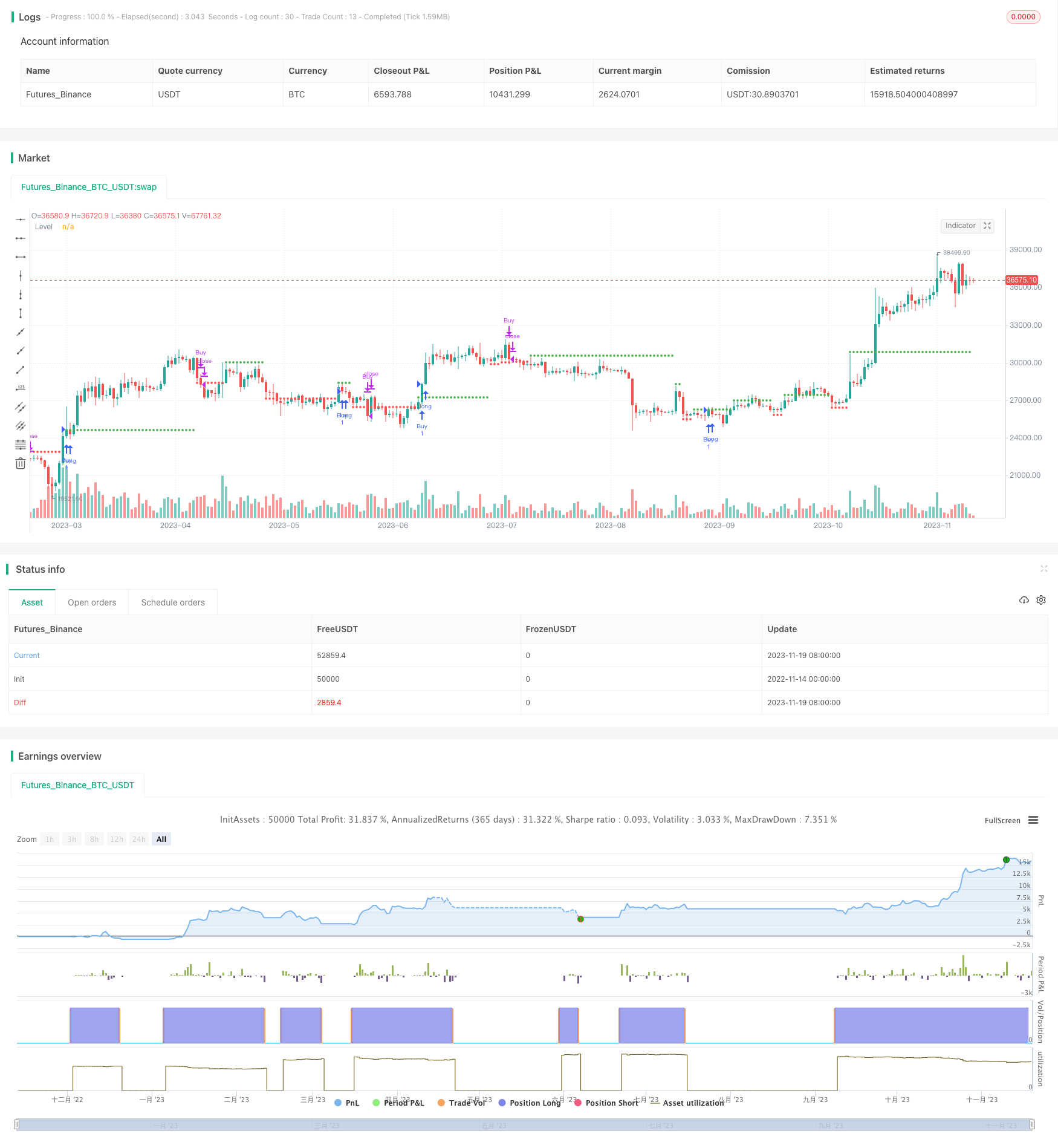
该策略通过计算多个技术指标的综合信号,判断当前时间框架下的趋势方向。当判断为上涨趋势时,在较高点设定追踪止损线;当判断为下跌趋势时,在较低点设定追踪止损线。策略可以自适应不同品种和不同时间框架,通过动态调整止损线,实现风险控制。
|
|
|
|
## 原理
|
|
|
|
该策略结合了均线、ATR、KD、变动率等多个指标,判断当前时间框架下的总体趋势方向。具体来说,它计算出以下几个子信号的综合值:
|
|
|
|
1. 均线方向信号
|
|
2. KD指标超买超卖信号
|
|
3. 量价背离信号
|
|
4. 通道突破信号
|
|
5. 多时间框架综合试错信号
|
|
6. Percent R信号
|
|
7. 均线回归信号
|
|
8. ATR通道突破信号
|
|
|
|
上述每个子信号都经过了平滑处理,并设定不同的阈值判断买入/卖出。 然后对每个子信号进行加权,计算出当前时间框架下的总体信号。如果信号大于0,则判断为上涨趋势,如果信号小于0,则判断为下跌趋势。
|
|
|
|
在判断为上涨趋势时,策略会在之前较高点附近设定追踪止损线;在判断为下跌趋势时,策略会在之前较低点附近设定追踪止损线。这样可以根据实际价格走势来动态调整止损位,实现风险控制的目的。
|
|
|
|
## 优势
|
|
|
|
该策略集成了多个指标判断当前趋势方向,提高了判断的准确性。同时,策略可以自适应不同品种和时间框架,具有较强的适应性。
|
|
|
|
最重要的是,该策略能够动态调整止损线,能够根据实际走势调整风险控制水平,从而对冲系统性风险,这是其最大的优势。
|
|
|
|
## 风险
|
|
|
|
该策略判断趋势信号的质量直接影响止损线的设定,如果判断产生错误,可能导致止损位设定过于宽松或过于严格。此外,止损线无法完全规避行情突变的风险。
|
|
|
|
该策略还需要权衡获利水平和止损距离,如果止损距离过近,可能导致止损过于频繁;如果止损距离过远,则无法有效控制风险。这需要根据不同品种不同周期进行参数优化。
|
|
|
|
## 优化方向
|
|
|
|
可以考虑引入机器学习算法,利用历史数据训练判断趋势方向的模型,从而提高判断准确性。
|
|
|
|
可以测试不同参数组合,优化止损线的距离。例如动态调整ATR周期参数,以适应市场波动率的变化。
|
|
|
|
还可以结合交易量能量指标判断真实趋势,防止量价背离导致的信号错误。
|
|
|
|
## 总结
|
|
|
|
该策略通过集成多个技术指标判断当前趋势方向,并据此动态调整追踪止损线,旨在提高止损的实效性,控制交易风险。该策略理念先进,值得进一步优化和验证,是一个可供参考的多时间框架自适应风险控制策略。
|
|
|
|
||
|
|
|
|
## Overview
|
|
|
|
This strategy calculates the comprehensive signals of multiple technical indicators to determine the trend direction in the current timeframe. When judged as an uptrend, a tracking stop loss line is set at a relatively high point; when judged as a downtrend, a tracking stop loss line is set at a relatively low point. The strategy can adaptively adjust the stop loss line to achieve risk control.
|
|
|
|
## Principle
|
|
|
|
The strategy combines multiple indicators such as moving averages, ATR, KD, and variance rate to determine the overall trend direction in the current timeframe. Specifically, it calculates the composite value of the following sub-signals:
|
|
|
|
1. Moving average direction signal
|
|
2. KD indicator overboughtoversold signal
|
|
3. Price-volume divergence signal
|
|
4. Channel breakthrough signal
|
|
5. Multi-timeframe combined trial-and-error signal
|
|
6. Percent R signal
|
|
7. Moving average regression signal
|
|
8. ATR channel breakthrough signal
|
|
|
|
Each sub-signal is smoothed and different thresholds are set to judge buy/sell. Then weight the sub-signals to calculate the overall signal in the current timeframe. If the signal is greater than 0, it is judged as an uptrend. If the signal is less than 0, it is judged as a downtrend.
|
|
|
|
When judged as an uptrend, the strategy sets a tracking stop loss line near the previous higher point; when judged as a downtrend, it sets a tracking stop loss line near the previous lower point. This can dynamically adjust the stop loss level according to the actual price movement to achieve the purpose of risk control.
|
|
|
|
## Advantages
|
|
|
|
The strategy integrates multiple indicators to judge the current trend direction, which improves the accuracy of judgment. At the same time, the strategy can adapt to different varieties and time frames with strong adaptability.
|
|
|
|
Most importantly, the strategy can dynamically adjust the stop loss line and adjust the risk control level according to the actual trend to hedge systemic risks. This is its biggest advantage.
|
|
|
|
## Risks
|
|
|
|
The quality of the trend signal judgment directly affects the setting of the stop loss line. If the judgment is wrong, it may cause the stop loss level to be set too loose or too strict. In addition, the stop loss line cannot completely avoid the risk of market mutations.
|
|
|
|
The strategy also needs to balance the profit level and the stop loss distance. If the stop loss distance is too close, it may cause excessive frequency of stop loss; if the stop loss distance is too far, it cannot effectively control risks. This requires parameter optimization for different varieties and cycles.
|
|
|
|
## Optimization Directions
|
|
|
|
Consider introducing machine learning algorithms to train models for judging trend directions using historical data to improve judgment accuracy.
|
|
|
|
Test different parameter combinations to optimize stop loss distance. For example, dynamically adjust ATR cycle parameters to adapt to changes in market volatility.
|
|
|
|
Volume energy indicators can also be combined to determine true trends and prevent signal errors caused by price-volume divergence.
|
|
|
|
## Summary
|
|
|
|
The strategy judges the current trend direction by integrating multiple technical indicators, and accordingly dynamically adjusts the tracking stop loss line. It aims to improve the effectiveness of stop loss and control trading risks. The strategy idea is advanced and worth further optimization and verification. It is a multi-timeframe adaptive risk control strategy that can be referenced.
|
|
|
|
[/trans]
|
|
|
|
> Strategy Arguments
|
|
|
|
|
|
|
|
|Argument|Default|Description|
|
|
|----|----|----|
|
|
|v_input_1|true|Run Back Testing|
|
|
|
|
|
|
> Source (PineScript)
|
|
|
|
``` pinescript
|
|
/*backtest
|
|
start: 2022-11-14 00:00:00
|
|
end: 2023-11-20 00:00:00
|
|
period: 1d
|
|
basePeriod: 1h
|
|
exchanges: [{"eid":"Futures_Binance","currency":"BTC_USDT"}]
|
|
*/
|
|
|
|
// This source code is subject to the terms of the Mozilla Public License 2.0 at https://mozilla.org/MPL/2.0/
|
|
// © jigneshjc
|
|
|
|
//@version=5
|
|
strategy("Jigga - Survival Level", shorttitle='Jigga - Survival Level', overlay=true)
|
|
|
|
doBackTesting = input(true, 'Run Back Testing')
|
|
|
|
entryCondition = false
|
|
exitCondition = false
|
|
|
|
|
|
ab21 = 14, gh41 = ab21
|
|
gh42 = ab21, ju51 = 14
|
|
ki61 = ju51
|
|
lkolkp = true ,ab22 = 58
|
|
cd31 = 5 , ab23 = 42
|
|
aa12 = 29, cd32 = 26
|
|
op71 = 5, aa11 = 12
|
|
aa13 = 9, op72 = 2.0
|
|
movnwx = false
|
|
|
|
|
|
kahachale(byju, h, l) =>
|
|
mika = ta.change(h)
|
|
awer = -ta.change(l)
|
|
uikmhDM = na(mika) ? na : mika > awer and mika > 0 ? mika : 0
|
|
wrtdfcDM = na(awer) ? na : awer > mika and awer > 0 ? awer : 0
|
|
bbct = ta.rma(ta.tr, byju)
|
|
uikmh = fixnan(100 * ta.rma(uikmhDM, byju) / bbct)
|
|
wrtdfc = fixnan(100 * ta.rma(wrtdfcDM, byju) / bbct)
|
|
[uikmh, wrtdfc]
|
|
|
|
trial(gh42, gh41, h, l) =>
|
|
[uikmh, wrtdfc] = kahachale(gh42, h, l)
|
|
uuolop = uikmh + wrtdfc
|
|
trial = 100 * ta.rma(math.abs(uikmh - wrtdfc) / (uuolop == 0 ? 1 : uuolop), gh41)
|
|
trial
|
|
|
|
_pr(src, byjugth) =>
|
|
max = ta.highest(byjugth)
|
|
min = ta.lowest(byjugth)
|
|
100 * (src - max) / (max - min)
|
|
|
|
|
|
kyukarna(khulmkhula, mikaarwala, nichewala, bandhwala, partiwala) =>
|
|
|
|
sig = trial(gh42, gh41, mikaarwala, nichewala)
|
|
trialIncreasing = sig > ta.ema(sig, 5) ? lkolkp : movnwx
|
|
|
|
rolkmn = ta.ema(bandhwala, aa11)
|
|
psolkmn = ta.ema(bandhwala, aa12)
|
|
ujghd = rolkmn - psolkmn
|
|
wrtycv = ta.ema(ujghd, aa13)
|
|
kimnjg = ujghd - wrtycv
|
|
|
|
|
|
mikalilo = ta.rma(math.max(ta.change(bandhwala), 0), ab21)
|
|
awerlilo = ta.rma(-math.min(ta.change(bandhwala), 0), ab21)
|
|
lilo = awerlilo == 0 ? 100 : mikalilo == 0 ? 0 : 100 - 100 / (1 + mikalilo / awerlilo)
|
|
juylknlilo = ta.ema(lilo, 3)
|
|
|
|
|
|
rjuylkn = ta.ema(bandhwala, cd31)
|
|
psjuylkn = ta.ema(bandhwala, cd32)
|
|
|
|
percentR = _pr(bandhwala, ju51)
|
|
juylknpercentR = ta.ema(percentR, 3)
|
|
|
|
|
|
ad = bandhwala == mikaarwala and bandhwala == nichewala or mikaarwala == nichewala ? 0 : (2 * bandhwala - nichewala - mikaarwala) / (mikaarwala - nichewala) * partiwala
|
|
kiloValue = math.sum(ad, ki61) / math.sum(partiwala, ki61)
|
|
|
|
|
|
|
|
liiopn = ta.atr(op71)
|
|
mikaliiopn = (mikaarwala + nichewala) / 2 - op72 * liiopn
|
|
mika1liiopn = nz(mikaliiopn[1], mikaliiopn)
|
|
mikaliiopn := bandhwala[1] > mika1liiopn ? math.max(mikaliiopn, mika1liiopn) : mikaliiopn
|
|
dnliiopn = (mikaarwala + nichewala) / 2 + op72 * liiopn
|
|
dn1liiopn = nz(dnliiopn[1], dnliiopn)
|
|
dnliiopn := bandhwala[1] < dn1liiopn ? math.min(dnliiopn, dn1liiopn) : dnliiopn
|
|
omnerliiopn = 1
|
|
omnerliiopn := nz(omnerliiopn[1], omnerliiopn)
|
|
omnerliiopn := omnerliiopn == -1 and bandhwala > dn1liiopn ? 1 : omnerliiopn == 1 and bandhwala < mika1liiopn ? -1 : omnerliiopn
|
|
|
|
fitur = ujghd > 0 ? ujghd > wrtycv ? 1 : 0 : ujghd > wrtycv ? 0 : -1
|
|
mitur = kimnjg >= 0 ? kimnjg > kimnjg[1] ? 1 : 0 : kimnjg > kimnjg[1] ? 0 : -1
|
|
ritur = juylknlilo > ab22 ? 1 : juylknlilo < ab23 ? -1 : 0
|
|
circuits = rjuylkn > psjuylkn ? 1 : -1
|
|
trialPoints = trialIncreasing ? close > ta.ema(close, 3) ? 1 : -1 : 0
|
|
virar = juylknpercentR > -ab23 ? 1 : juylknpercentR < -ab22 ? -1 : 0
|
|
chikar = kiloValue > 0.1 ? 1 : kiloValue < -0.1 ? -1 : 0
|
|
sitar = omnerliiopn
|
|
|
|
|
|
p = fitur + mitur + ritur + circuits + trialPoints + virar + chikar + sitar
|
|
|
|
p
|
|
|
|
currentP = kyukarna(open, high, low, close, volume)
|
|
currentPNew = currentP >= 0 and currentP[1] <= 0 ? 0 : currentP <= 0 and currentP[1] >= 0 ? 0 : currentP
|
|
colorPNew = currentPNew == 0 ? color.black : currentPNew >= 0 ? color.green : color.red
|
|
//plot(currentPNew, color=colorPNew, title='CurrentTimeFrame')
|
|
|
|
LTN = 0.0
|
|
LTN := nz(LTN) ? 0.0 : (currentPNew[1] < 0 and currentPNew >= 0) ? high * 1.005 : (currentPNew[1] > 0 and currentPNew <= 0) ? low * 0.995 : LTN[1]
|
|
|
|
LClr = color.green
|
|
LClr := (currentPNew[1] < 0 and currentPNew >= 0) ? color.green : (currentPNew[1] > 0 and currentPNew <= 0) ? color.red : LClr[1]
|
|
|
|
plot(LTN,color=LClr,title="Level", style=plot.style_circles)
|
|
|
|
|
|
entryCondition:= high > LTN and LClr == color.green ? lkolkp : movnwx
|
|
exitCondition:= low < LTN and LClr == color.red ? lkolkp : movnwx
|
|
|
|
tradeRunning = movnwx
|
|
tradeRunning := nz(tradeRunning) ? movnwx : (not tradeRunning[1]) and entryCondition ? lkolkp : tradeRunning[1] and exitCondition ? movnwx : tradeRunning[1]
|
|
|
|
|
|
plotshape(tradeRunning and (not tradeRunning[1]) and (not doBackTesting), style=shape.labelup, location=location.belowbar, color=color.new(#00FF00, 50), size=size.tiny, title='Buy wrtycv', text='➹', textcolor=color.new(color.black,0))
|
|
plotshape((not tradeRunning) and tradeRunning[1] and (not doBackTesting), style=shape.labeldown, location=location.abovebar, color=color.new(#FF0000, 50), size=size.tiny, title='Sell wrtycv', text='➷', textcolor=color.new(color.white, 0))
|
|
|
|
|
|
if entryCondition and doBackTesting
|
|
strategy.entry(id="Buy",direction=strategy.long)
|
|
|
|
if exitCondition and doBackTesting
|
|
strategy.close(id="Buy")
|
|
|
|
|
|
```
|
|
|
|
> Detail
|
|
|
|
https://www.fmz.com/strategy/432754
|
|
|
|
> Last Modified
|
|
|
|
2023-11-21 11:07:44
|