
252 lines
17 KiB
Markdown
252 lines
17 KiB
Markdown
|
|
> Name
|
|
|
|
小时周期价格开口策略追踪开盘与收盘价差的智能对比量化交易系统-Hourly-Open-Close-Price-Differential-Smart-Comparison-Quantitative-Trading-System
|
|
|
|
> Author
|
|
|
|
ianzeng123
|
|
|
|
> Strategy Description
|
|
|
|
|
|
|
|
|
|
|
|
|
|
[trans]
|
|
|
|
## 概述
|
|
|
|
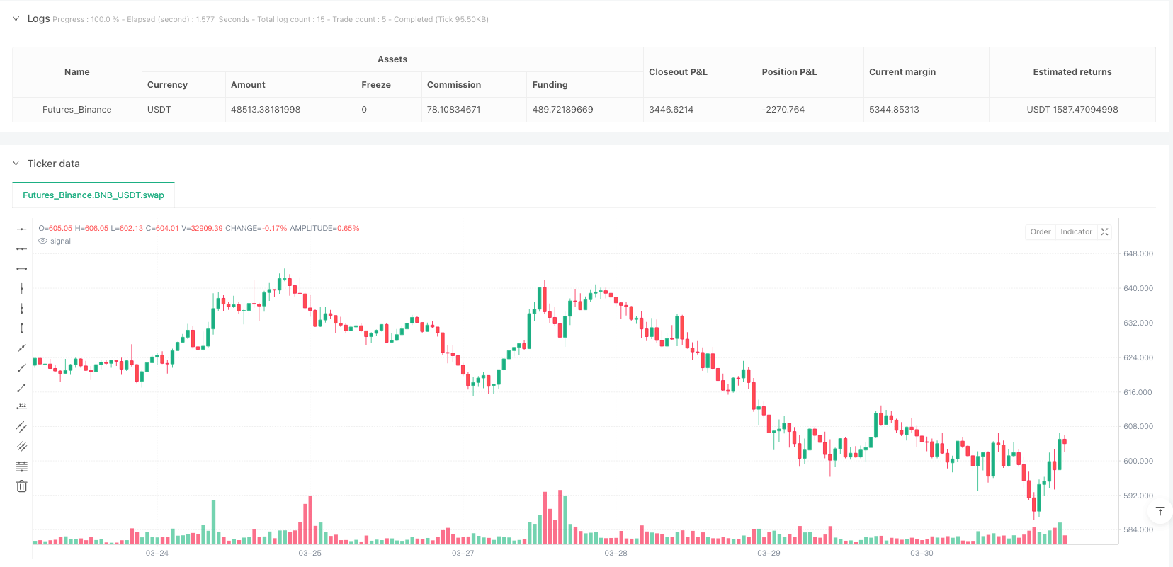
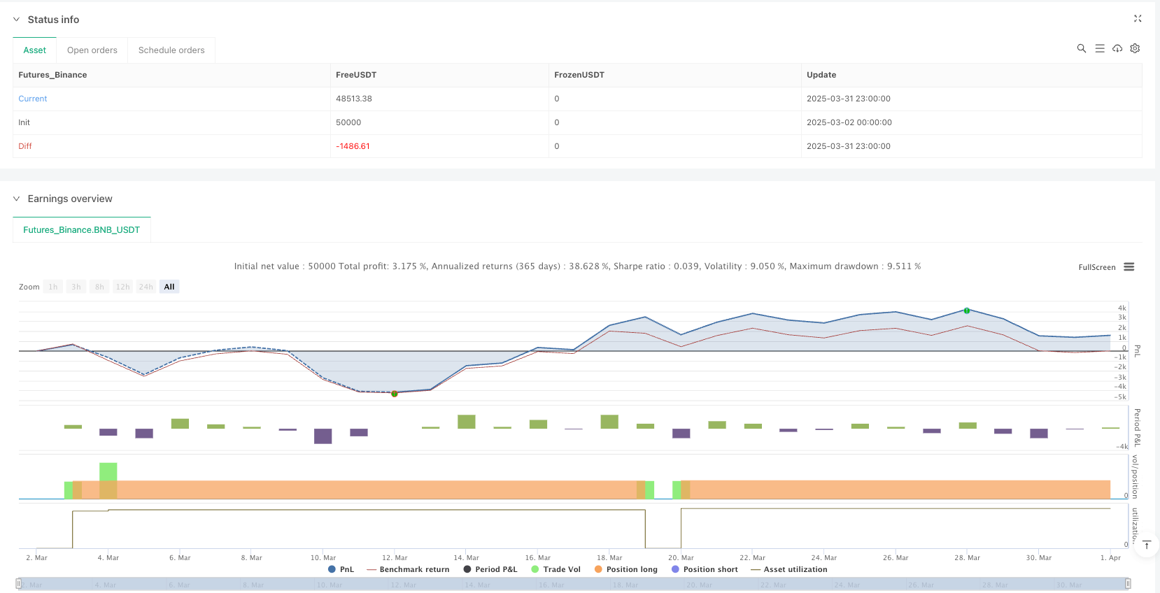
小时周期价格开口策略是一种基于价格行为分析的量化交易系统,专注于捕捉市场开盘价与前一周期收盘价之间的动量变化。该策略通过比较当前周期的开盘价与前一周期的收盘价来识别潜在的价格上涨趋势,并在满足特定条件时建立多头头寸。系统设置了固定百分比的利润目标(3%),一旦达到目标价格,策略自动平仓,锁定利润。该策略的核心优势在于其简单性和可执行性,使其成为短期交易者和日内交易者的理想选择。
|
|
|
|
## 策略原理
|
|
|
|
小时周期价格开口策略的核心原理基于市场价格行为和动量理论。具体来说,该策略遵循以下逻辑流程:
|
|
|
|
1. 买入条件判断:策略首先检查当前周期的开盘价是否高于前一周期的收盘价(open > close[1]),同时确保当前没有持仓(strategy.position_size == 0)。这两个条件同时满足时,系统识别为买入信号。
|
|
|
|
2. 执行买入订单:当买入条件满足时,系统通过strategy.entry("Buy", strategy.long)命令执行多头入场。同时,在价格图表上标记买入点位,显示具体的买入价格。
|
|
|
|
3. 设定利润目标:入场后,系统立即计算利润目标价格,设定为买入价格的103%(targetPrice = strategy.position_avg_price * 1.03),相当于3%的止盈水平。
|
|
|
|
4. 平仓条件监控:策略持续监控当前市场价格,一旦收盘价达到或超过目标价格(close >= targetPrice),且持有多头头寸(strategy.position_size > 0),系统自动执行平仓操作。
|
|
|
|
5. 可视化交易:为了直观地展示交易活动,策略在图表上绘制买入和卖出信号,使交易者能够清晰地跟踪策略执行情况。
|
|
|
|
该策略利用了价格动量的延续性原理,当开盘价高于前一周期收盘价时,往往意味着市场存在上涨动能,这种动能可能会在短期内持续,从而带来获利机会。
|
|
|
|
## 策略优势
|
|
|
|
深入分析该策略的代码实现,可以总结出以下显著优势:
|
|
|
|
1. 简洁明了的入场逻辑:策略使用简单且易于理解的价格比较作为入场信号,不依赖复杂的指标或参数设置,降低了过度拟合的风险。
|
|
|
|
2. 明确的利润目标:固定3%的止盈设置提供了清晰的利润预期,有助于维持良好的风险回报比。
|
|
|
|
3. 自动化执行:策略完全自动化,从信号识别到入场再到平仓,减少了人为干预和情绪决策的影响。
|
|
|
|
4. 资金管理整合:通过default_qty_type=strategy.percent_of_equity和default_qty_value=100参数设置,策略在每次交易中投入账户总价值的100%,简化了资金管理。
|
|
|
|
5. 可视化交易记录:通过在图表上标记买入和卖出点位,交易者可以直观地审查策略执行情况,有助于后续分析和策略调整。
|
|
|
|
6. 防止重复入场:通过检查当前持仓状态(strategy.position_size == 0),策略确保在已有持仓的情况下不会重复入场,避免了不必要的风险累积。
|
|
|
|
7. 适用于高流动性市场:策略在小时时间框架上运行,特别适合流动性较高的市场环境,确保了交易信号的可执行性。
|
|
|
|
## 策略风险
|
|
|
|
尽管该策略设计简洁,但仍存在一些潜在风险:
|
|
|
|
1. 缺乏止损机制:当前策略仅设置了止盈条件,没有明确的止损机制。如果市场朝不利方向发展,可能导致较大损失。建议添加止损条件,例如基于时间或价格的止损设置。
|
|
|
|
2. 固定百分比目标的局限性:3%的固定止盈目标可能无法适应不同市场环境和波动性。在低波动市场中可能过高,而在高波动市场中则可能过低。
|
|
|
|
3. 单一入场条件的脆弱性:仅依赖开盘价与前一周期收盘价的比较作为入场信号,可能导致在市场噪音较大时产生误导信号。
|
|
|
|
4. 缺乏趋势过滤:策略没有考虑更广泛的市场趋势环境,可能在下降趋势中也发出买入信号,增加了逆势交易风险。
|
|
|
|
5. 资金管理风险:默认使用100%账户权益进行交易,没有根据市场波动性或风险水平调整仓位大小,可能导致风险过度集中。
|
|
|
|
6. 时间框架依赖:策略专注于小时周期,可能无法捕捉更短时间框架内的价格波动或更长期的市场趋势。
|
|
|
|
7. 回测偏差风险:使用收盘价作为触发平仓的条件可能在实际交易中导致执行滑点,因为实际中可能需要等到收盘价确认才能执行。
|
|
|
|
## 策略优化方向
|
|
|
|
基于对策略代码的深入分析,我们可以提出以下优化方向:
|
|
|
|
1. 引入止损机制:添加基于时间或价格的止损条件,例如设置最大持仓时间或基于ATR(真实波动幅度)的止损水平,以限制单笔交易的最大亏损。
|
|
|
|
2. 动态利润目标:将固定的3%止盈目标改为基于市场波动性的动态目标,例如使用ATR的倍数作为目标价格计算基础。
|
|
|
|
3. 增加入场过滤条件:结合其他技术指标(如移动平均线、RSI或MACD)作为确认信号,提高入场信号的质量和可靠性。
|
|
|
|
4. 添加趋势方向过滤:引入长期移动平均线或其他趋势指标,确保只在整体趋势方向一致的情况下入场。
|
|
|
|
5. 优化资金管理:实施动态仓位管理,根据市场状况、账户权益和风险水平调整每次交易的资金比例。
|
|
|
|
6. 多时间框架分析:整合更高时间框架的市场分析结果,只在高低时间框架趋势一致的情况下执行交易。
|
|
|
|
7. 引入时间过滤:添加交易时间窗口限制,避开波动性过低或过高的市场时段。
|
|
|
|
8. 优化执行逻辑:考虑使用限价单而非市价单执行交易,减少滑点和执行成本。
|
|
|
|
这些优化方向的实施将有助于提高策略的稳健性和适应性,使其能够在不同市场环境中保持相对稳定的表现。
|
|
|
|
## 总结
|
|
|
|
小时周期价格开口策略是一个简洁而实用的交易系统,利用开盘价与前一周期收盘价之间的关系捕捉短期价格动量。该策略以其简单的逻辑和明确的执行规则,为交易者提供了一种容易理解和实施的交易方法。尽管存在一些潜在风险,如缺乏止损机制和单一入场条件的局限性,但通过引入止损策略、动态利润目标设置和额外的入场过滤条件等优化措施,可以显著提升策略的稳健性和盈利潜力。
|
|
|
|
该策略特别适合短期交易者和日内交易者,尤其是在波动性适中的市场环境中。通过持续的回测和优化,交易者可以根据特定市场和个人风险偏好调整参数,进一步提高策略表现。最终,无论是作为独立交易系统还是作为更复杂交易策略的组成部分,小时周期价格开口策略都展示了基于价格行为分析的量化交易方法的潜力和价值。 ||
|
|
|
|
## Overview
|
|
|
|
The Hourly Open-Close Price Differential Smart Comparison Quantitative Trading System is a price action-based quantitative trading strategy that focuses on capturing momentum shifts between the current period's open price and the previous period's close price. The strategy identifies potential upward price trends by comparing the current period's opening price with the previous period's closing price, establishing long positions when specific conditions are met. The system incorporates a fixed percentage profit target (3%), automatically closing positions when the target price is reached to secure profits. The core advantage of this strategy lies in its simplicity and executability, making it an ideal choice for short-term traders and intraday traders.
|
|
|
|
## Strategy Principles
|
|
|
|
The Hourly Open-Close Price Differential strategy is based on market price action and momentum theory. Specifically, the strategy follows this logical process:
|
|
|
|
1. Buy Condition Evaluation: The strategy first checks if the current period's opening price is higher than the previous period's closing price (open > close[1]), while ensuring no current position exists (strategy.position_size == 0). When both conditions are satisfied, the system identifies a buy signal.
|
|
|
|
2. Buy Order Execution: When the buy condition is met, the system executes a long entry through the strategy.entry("Buy", strategy.long) command. Simultaneously, it marks the buy point on the price chart, displaying the specific entry price.
|
|
|
|
3. Profit Target Setting: After entry, the system immediately calculates the profit target price, set at 103% of the purchase price (targetPrice = strategy.position_avg_price * 1.03), equivalent to a 3% take-profit level.
|
|
|
|
4. Exit Condition Monitoring: The strategy continuously monitors the current market price, and once the closing price reaches or exceeds the target price (close >= targetPrice) while holding a long position (strategy.position_size > 0), the system automatically executes the closing operation.
|
|
|
|
5. Trade Visualization: To intuitively display trading activity, the strategy plots buy and sell signals on the chart, allowing traders to clearly track strategy execution.
|
|
|
|
This strategy leverages the principle of price momentum continuity, where an opening price higher than the previous period's closing price often indicates market upward momentum that may continue in the short term, creating profit opportunities.
|
|
|
|
## Strategy Advantages
|
|
|
|
Through deep analysis of the strategy's code implementation, the following significant advantages can be summarized:
|
|
|
|
1. Clear and Concise Entry Logic: The strategy uses a simple and easy-to-understand price comparison as the entry signal, without relying on complex indicators or parameter settings, reducing the risk of overfitting.
|
|
|
|
2. Defined Profit Targets: The fixed 3% take-profit setting provides clear profit expectations, helping to maintain a good risk-reward ratio.
|
|
|
|
3. Automated Execution: The strategy is fully automated from signal identification to entry and exit, reducing human intervention and emotional decision-making.
|
|
|
|
4. Integrated Fund Management: Through default_qty_type=strategy.percent_of_equity and default_qty_value=100 parameter settings, the strategy invests 100% of the account value in each trade, simplifying fund management.
|
|
|
|
5. Visualized Trading Records: By marking buy and sell points on the chart, traders can visually review strategy execution, facilitating subsequent analysis and strategy adjustments.
|
|
|
|
6. Prevention of Duplicate Entries: By checking the current position status (strategy.position_size == 0), the strategy ensures no re-entry when a position already exists, avoiding unnecessary risk accumulation.
|
|
|
|
7. Suitability for High Liquidity Markets: The strategy operates on an hourly timeframe, particularly suitable for high liquidity market environments, ensuring the executability of trading signals.
|
|
|
|
## Strategy Risks
|
|
|
|
Despite the strategy's concise design, there are several potential risks:
|
|
|
|
1. Lack of Stop-Loss Mechanism: The current strategy only sets take-profit conditions without a clear stop-loss mechanism. If the market moves unfavorably, it could lead to significant losses. It is recommended to add stop-loss conditions, such as time-based or price-based stop-loss settings.
|
|
|
|
2. Limitations of Fixed Percentage Targets: The fixed 3% take-profit target may not adapt to different market environments and volatilities. It may be too high in low-volatility markets and too low in high-volatility markets.
|
|
|
|
3. Vulnerability of Single Entry Condition: Relying solely on the comparison between opening price and previous period's closing price as an entry signal may lead to misleading signals when market noise is significant.
|
|
|
|
4. Lack of Trend Filtering: The strategy does not consider the broader market trend environment and may issue buy signals even in downtrends, increasing the risk of counter-trend trading.
|
|
|
|
5. Fund Management Risk: The default uses 100% of account equity for trading without adjusting position size based on market volatility or risk level, potentially leading to excessive risk concentration.
|
|
|
|
6. Timeframe Dependence: The strategy focuses on the hourly period and may fail to capture price fluctuations in shorter timeframes or longer-term market trends.
|
|
|
|
7. Backtest Bias Risk: Using the closing price as a trigger for closing positions may lead to execution slippage in actual trading, as one might need to wait for closing price confirmation before execution.
|
|
|
|
## Strategy Optimization Directions
|
|
|
|
Based on in-depth analysis of the strategy code, we can propose the following optimization directions:
|
|
|
|
1. Introduce Stop-Loss Mechanism: Add time-based or price-based stop-loss conditions, such as setting maximum holding time or ATR-based (Average True Range) stop-loss levels to limit maximum loss per trade.
|
|
|
|
2. Dynamic Profit Targets: Change the fixed 3% take-profit target to a volatility-based dynamic target, such as using multiples of ATR as the basis for target price calculation.
|
|
|
|
3. Add Entry Filtering Conditions: Combine other technical indicators (such as moving averages, RSI, or MACD) as confirmation signals to improve the quality and reliability of entry signals.
|
|
|
|
4. Add Trend Direction Filtering: Introduce long-term moving averages or other trend indicators to ensure entries only when the overall trend direction is consistent.
|
|
|
|
5. Optimize Fund Management: Implement dynamic position management, adjusting the proportion of funds for each trade based on market conditions, account equity, and risk levels.
|
|
|
|
6. Multi-Timeframe Analysis: Integrate market analysis results from higher timeframes, executing trades only when trends across different timeframes align.
|
|
|
|
7. Introduce Time Filtering: Add trading time window restrictions to avoid market periods with too low or too high volatility.
|
|
|
|
8. Optimize Execution Logic: Consider using limit orders instead of market orders to execute trades, reducing slippage and execution costs.
|
|
|
|
Implementing these optimization directions will help improve the strategy's robustness and adaptability, enabling it to maintain relatively stable performance across different market environments.
|
|
|
|
## Summary
|
|
|
|
The Hourly Open-Close Price Differential Smart Comparison Quantitative Trading System is a concise and practical trading system that captures short-term price momentum by utilizing the relationship between opening prices and previous period closing prices. With its simple logic and clear execution rules, the strategy provides traders with an easy-to-understand and implement trading method. Despite some potential risks, such as the lack of a stop-loss mechanism and limitations of single entry conditions, the strategy's robustness and profit potential can be significantly enhanced through optimizations like introducing stop-loss strategies, dynamic profit target settings, and additional entry filtering conditions.
|
|
|
|
This strategy is particularly suitable for short-term traders and day traders, especially in markets with moderate volatility. Through continuous backtesting and optimization, traders can adjust parameters according to specific markets and personal risk preferences to further improve strategy performance. Ultimately, whether as an independent trading system or as a component of more complex trading strategies, the Hourly Open-Close Price Differential strategy demonstrates the potential and value of quantitative trading methods based on price action analysis.[/trans]
|
|
|
|
|
|
|
|
> Source (PineScript)
|
|
|
|
``` pinescript
|
|
/*backtest
|
|
start: 2025-03-02 00:00:00
|
|
end: 2025-04-01 00:00:00
|
|
period: 1h
|
|
basePeriod: 1h
|
|
exchanges: [{"eid":"Futures_Binance","currency":"BNB_USDT"}]
|
|
*/
|
|
|
|
//@version=6
|
|
|
|
strategy("1 Hour Open vs Close Buy Strategy", overlay=true, default_qty_type=strategy.percent_of_equity, default_qty_value=100)
|
|
|
|
|
|
|
|
// Define the buy condition: current open is higher than the previous close
|
|
|
|
buyCondition = open > close[1] and strategy.position_size == 0 // Only buy if there is no active position
|
|
|
|
|
|
|
|
// Execute the buy order and plot buy price
|
|
|
|
if (buyCondition)
|
|
|
|
strategy.entry("Buy", strategy.long)
|
|
|
|
label.new(x=bar_index, y=low, text="Buy at: " + str.tostring(open), style=label.style_label_up, color=color.green, size=size.normal, textcolor=color.white)
|
|
|
|
|
|
|
|
// Define the sell condition based on 3% profit target from the buy price
|
|
|
|
targetPrice = strategy.position_avg_price * 1.03
|
|
|
|
|
|
|
|
// Check if the current price has reached the target price and close the position
|
|
|
|
if (strategy.position_size > 0 and close >= targetPrice)
|
|
|
|
strategy.close("Buy")
|
|
|
|
label.new(x=bar_index, y=high, text="Sell at: " + str.tostring(close), style=label.style_label_down, color=color.red, size=size.normal, textcolor=color.white)
|
|
|
|
|
|
|
|
// Plotting to visualize entries and exits on the chart
|
|
|
|
plotshape(series=buyCondition, location=location.belowbar, color=color.green, style=shape.labelup, text="Buy")
|
|
|
|
plotshape(series=(strategy.position_size > 0 and close >= targetPrice), location=location.abovebar, color=color.red, style=shape.labeldown, text="Sell")
|
|
```
|
|
|
|
> Detail
|
|
|
|
https://www.fmz.com/strategy/489153
|
|
|
|
> Last Modified
|
|
|
|
2025-04-02 11:15:52
|