
405 lines
12 KiB
Markdown
405 lines
12 KiB
Markdown
|
|
> Name
|
|
|
|
基于时间序列分解和成交量加权的布林带技术指标策略Trend-Following-Strategy-Based-on-Time-Series-Decomposition-and-Volume-Weighted-Bollinger-Bands
|
|
|
|
> Author
|
|
|
|
ChaoZhang
|
|
|
|
> Strategy Description
|
|
|
|
|
|
[trans]
|
|
## 概述
|
|
|
|
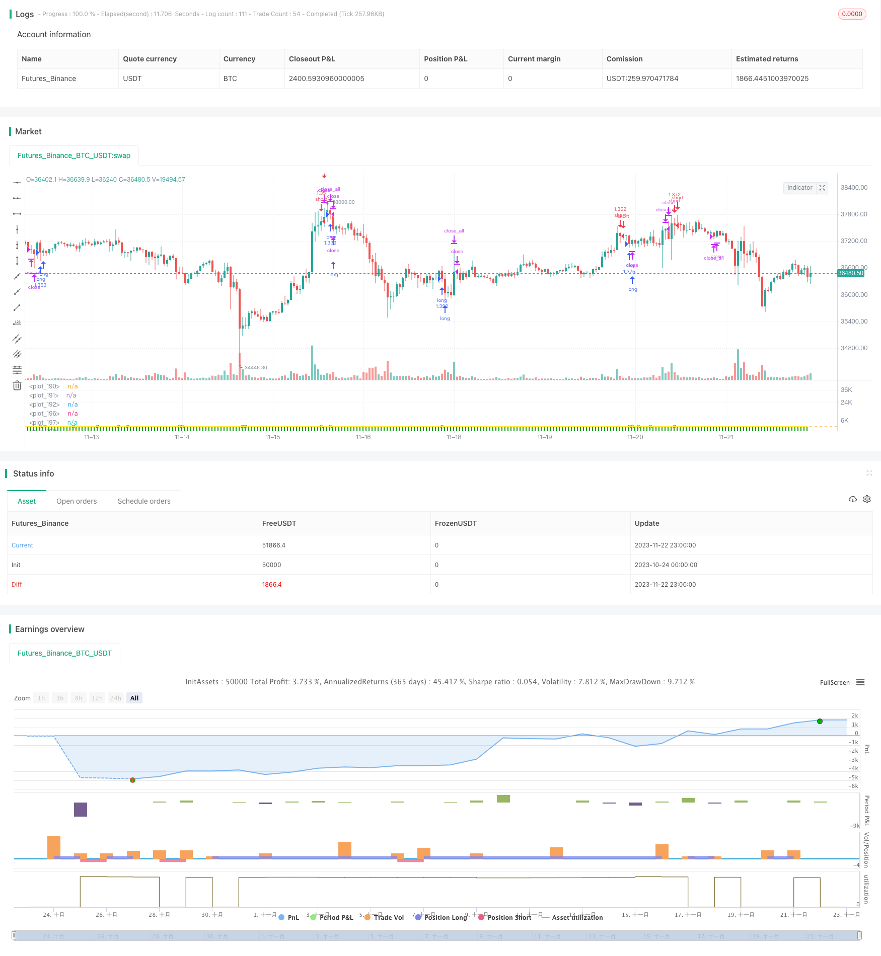
该策略融合了时间序列分解、成交量加权平均价、布林带和 delta(OBV-PVT) 4种技术指标,以实现对价格趋势、超买超卖的多维度判断。
|
|
|
|
## 策略原理
|
|
|
|
1. 使用时间序列分解去除价格中的噪音和周期性,得到更为准确的趋势判断;
|
|
2. 基于该趋势线,计算成交量加权后的新价格;
|
|
3. 计算收盘价的布林带百分比宽度BB%B指标来判断超买超卖;
|
|
4. 计算OBV-PVT的变化量Delta(OBV-PVT)的布林带百分比宽度,作为量价背离的判断标准;
|
|
5. 根据量价指标的多空交叉以及布林带指标的过冲回撤来产生交易信号。
|
|
|
|
## 优势分析
|
|
|
|
1. 结合了价格、成交量和统计特征的多重判断,策略健壮性好;
|
|
2. BB%B和Delta(OBV-PVT)相结合,能更好地判断短期的超买超卖现象;
|
|
3. 量价交叉信号过滤了部分噪音交易点。
|
|
|
|
## 风险分析
|
|
|
|
1. 参数设置过于复杂,不易调整;
|
|
2. 短期区间震荡可能增加损失;
|
|
3. 量价背离并不能完全过滤误导信号。
|
|
|
|
可以通过调整均线周期、布林带幅度以及风险盈亏比来优化策略,降低交易频率的同时提高单次交易的盈亏比。
|
|
|
|
## 总结
|
|
|
|
该策略综合运用了时间序列分解、布林带指标、OBV指标等多种分析工具,通过量价关系、统计特性以及趋势判断的有机结合,实现对短期余震的识别,能有效抓住市场的主要趋势。同时也存在一定的风险,需要通过参数调整以达到最优状态。
|
|
|
|
||
|
|
|
|
## Overview
|
|
|
|
This strategy integrates time series decomposition, volume weighted average price, Bollinger Bands and delta(OBV-PVT) 4 technical indicators to make multidimensional judgments on price trends, overbought and oversold conditions.
|
|
|
|
## Principles
|
|
|
|
1. Use time series decomposition to remove noise and periodicity in prices for more accurate trend judgment;
|
|
2. Calculate volume weighted new price based on the trend line;
|
|
3. Calculate the Bollinger Bands Percentage Width (BB%B) of closing price to determine overbought and oversold conditions;
|
|
4. Calculate the BB%B of Delta(OBV-PVT) as a measure of price-volume divergence;
|
|
5. Generate trading signals based on price-volume indicators crosses and Bollinger Bands overshoots and undershoots.
|
|
|
|
## Advantages
|
|
|
|
1. Combines price, volume and statistical features for robust judgments;
|
|
2. BB%B combined with Delta(OBV-PVT) better identifies short-term overbought/oversold conditions;
|
|
3. Price-volume crossover signals filter out some false signals.
|
|
|
|
## Risks
|
|
|
|
1. Too complex parameter tuning;
|
|
2. Short-term choppiness may increase losses;
|
|
3. Price-volume divergences do not completely filter false signals.
|
|
|
|
Parameters like moving averages, Bollinger Bands widths and risk-reward ratios can be optimized to reduce trading frequency while improving risk-adjusted returns per trade.
|
|
|
|
## Conclusion
|
|
|
|
Integrating tools like time series decomposition, Bollinger Bands, OBV indicators, this strategy combines price-volume relationships, statistical properties and trend analysis to identify short-term reversals and catch major trends. There are also certain risks that need to be addressed through parameter tuning for optimal performance.
|
|
|
|
[/trans]
|
|
|
|
> Strategy Arguments
|
|
|
|
|
|
|
|
|Argument|Default|Description|
|
|
|----|----|----|
|
|
|v_input_1|true|Start Date|
|
|
|v_input_2|true|Start Month|
|
|
|v_input_3|2010|Start Year|
|
|
|v_input_4|31|End Date|
|
|
|v_input_5|12|End Month|
|
|
|v_input_6|2021|End Year|
|
|
|v_input_7|2|Stop Loss %|
|
|
|v_input_8|4|Take Profit %|
|
|
|v_input_9|20|length|
|
|
|v_input_10|2|StdDev|
|
|
|v_input_11|1000|Smoothing Factor (Lambda)|
|
|
|v_input_12|100|Filter Length|
|
|
|v_input_13|1|TimeFrame|
|
|
|v_input_14|false|Show barcolors|
|
|
|v_input_15|false|Show previous VWAP close|
|
|
|v_input_16|20|l1|
|
|
|v_input_17|2|StdDev|
|
|
|v_input_18|0.3|xx|
|
|
|v_input_19|0.7|yy|
|
|
|v_input_20|-1|zz|
|
|
|v_input_21|16|Period|
|
|
|
|
|
|
> Source (PineScript)
|
|
|
|
``` pinescript
|
|
/*backtest
|
|
start: 2023-10-24 00:00:00
|
|
end: 2023-11-23 00:00:00
|
|
period: 1h
|
|
basePeriod: 15m
|
|
exchanges: [{"eid":"Futures_Binance","currency":"BTC_USDT"}]
|
|
*/
|
|
|
|
// This source code is subject to the terms of the Mozilla Public License 2.0 at https://mozilla.org/MPL/2.0/
|
|
//// This source code is subject to the terms of the Mozilla Public License 2.0 at https://mozilla.org/MPL/2.0/
|
|
// © oakwhiz and tathal
|
|
|
|
//@version=4
|
|
strategy("BBPBΔ(OBV-PVT)BB", default_qty_type=strategy.percent_of_equity, default_qty_value=100)
|
|
|
|
startDate = input(title="Start Date", type=input.integer,
|
|
defval=1, minval=1, maxval=31)
|
|
startMonth = input(title="Start Month", type=input.integer,
|
|
defval=1, minval=1, maxval=12)
|
|
startYear = input(title="Start Year", type=input.integer,
|
|
defval=2010, minval=1800, maxval=2100)
|
|
|
|
endDate = input(title="End Date", type=input.integer,
|
|
defval=31, minval=1, maxval=31)
|
|
endMonth = input(title="End Month", type=input.integer,
|
|
defval=12, minval=1, maxval=12)
|
|
endYear = input(title="End Year", type=input.integer,
|
|
defval=2021, minval=1800, maxval=2100)
|
|
|
|
// Normalize Function
|
|
normalize(_src, _min, _max) =>
|
|
// Normalizes series with unknown min/max using historical min/max.
|
|
// _src : series to rescale.
|
|
// _min, _min: min/max values of rescaled series.
|
|
var _historicMin = 10e10
|
|
var _historicMax = -10e10
|
|
_historicMin := min(nz(_src, _historicMin), _historicMin)
|
|
_historicMax := max(nz(_src, _historicMax), _historicMax)
|
|
_min + (_max - _min) * (_src - _historicMin) / max(_historicMax - _historicMin, 10e-10)
|
|
|
|
|
|
// STEP 2:
|
|
// Look if the close time of the current bar
|
|
// falls inside the date range
|
|
inDateRange = true
|
|
|
|
|
|
// Stop loss & Take Profit Section
|
|
sl_inp = input(2.0, title='Stop Loss %')/100
|
|
tp_inp = input(4.0, title='Take Profit %')/100
|
|
|
|
stop_level = strategy.position_avg_price * (1 - sl_inp)
|
|
take_level = strategy.position_avg_price * (1 + tp_inp)
|
|
|
|
icreturn = false
|
|
innercandle = if (high < high[1]) and (low > low[1])
|
|
icreturn := true
|
|
|
|
src = close
|
|
|
|
float change_src = change(src)
|
|
float i_obv = cum(change_src > 0 ? volume : change_src < 0 ? -volume : 0*volume)
|
|
float i_pvt = pvt
|
|
|
|
float result = change(i_obv - i_pvt)
|
|
|
|
float nresult = ema(normalize(result, -1, 1), 20)
|
|
|
|
|
|
|
|
length = input(20, minval=1)
|
|
mult = input(2.0, minval=0.001, maxval=50, title="StdDev")
|
|
basis = ema(nresult, length)
|
|
dev = mult * stdev(nresult, length)
|
|
upper = basis + dev
|
|
lower = basis - dev
|
|
bbr = (nresult - lower)/(upper - lower)
|
|
|
|
|
|
|
|
////////////////INPUTS///////////////////
|
|
lambda = input(defval = 1000, type = input.float, title = "Smoothing Factor (Lambda)", minval = 1)
|
|
leng = input(defval = 100, type = input.integer, title = "Filter Length", minval = 1)
|
|
srcc = close
|
|
|
|
///////////Construct Arrays///////////////
|
|
a = array.new_float(leng, 0.0)
|
|
b = array.new_float(leng, 0.0)
|
|
c = array.new_float(leng, 0.0)
|
|
d = array.new_float(leng, 0.0)
|
|
e = array.new_float(leng, 0.0)
|
|
f = array.new_float(leng, 0.0)
|
|
|
|
/////////Initialize the Values///////////
|
|
//for more details visit:
|
|
// https://asmquantmacro.com/2015/06/25/hodrick-prescott-filter-in-excel/
|
|
|
|
ll1 = leng-1
|
|
ll2 = leng-2
|
|
|
|
for i = 0 to ll1
|
|
array.set(a,i, lambda*(-4))
|
|
array.set(b,i, src[i])
|
|
array.set(c,i, lambda*(-4))
|
|
array.set(d,i, lambda*6 + 1)
|
|
array.set(e,i, lambda)
|
|
array.set(f,i, lambda)
|
|
|
|
array.set(d, 0, lambda + 1.0)
|
|
array.set(d, ll1, lambda + 1.0)
|
|
array.set(d, 1, lambda * 5.0 + 1.0)
|
|
array.set(d, ll2, lambda * 5.0 + 1.0)
|
|
|
|
array.set(c, 0 , lambda * (-2.0))
|
|
array.set(c, ll2, lambda * (-2.0))
|
|
|
|
array.set(a, 0 , lambda * (-2.0))
|
|
array.set(a, ll2, lambda * (-2.0))
|
|
|
|
//////////////Solve the optimization issue/////////////////////
|
|
float r = array.get(a, 0)
|
|
float s = array.get(a, 1)
|
|
float t = array.get(e, 0)
|
|
float xmult = 0.0
|
|
|
|
for i = 1 to ll2
|
|
xmult := r / array.get(d, i-1)
|
|
array.set(d, i, array.get(d, i) - xmult * array.get(c, i-1))
|
|
array.set(c, i, array.get(c, i) - xmult * array.get(f, i-1))
|
|
array.set(b, i, array.get(b, i) - xmult * array.get(b, i-1))
|
|
|
|
xmult := t / array.get(d, i-1)
|
|
r := s - xmult*array.get(c, i-1)
|
|
array.set(d, i+1, array.get(d, i+1) - xmult * array.get(f, i-1))
|
|
array.set(b, i+1, array.get(b, i+1) - xmult * array.get(b, i-1))
|
|
|
|
s := array.get(a, i+1)
|
|
t := array.get(e, i)
|
|
|
|
xmult := r / array.get(d, ll2)
|
|
array.set(d, ll1, array.get(d, ll1) - xmult * array.get(c, ll2))
|
|
|
|
x = array.new_float(leng, 0)
|
|
array.set(x, ll1, (array.get(b, ll1) - xmult * array.get(b, ll2)) / array.get(d, ll1))
|
|
array.set(x, ll2, (array.get(b, ll2) - array.get(c, ll2) * array.get(x, ll1)) / array.get(d, ll2))
|
|
|
|
for j = 0 to leng-3
|
|
i = leng-3 - j
|
|
array.set(x, i, (array.get(b,i) - array.get(f,i)*array.get(x,i+2) - array.get(c,i)*array.get(x,i+1)) / array.get(d, i))
|
|
|
|
|
|
|
|
//////////////Construct the output///////////////////
|
|
o5 = array.get(x,0)
|
|
|
|
////////////////////Plottingd///////////////////////
|
|
|
|
|
|
|
|
TimeFrame = input('1', type=input.resolution)
|
|
start = security(syminfo.tickerid, TimeFrame, time)
|
|
|
|
//------------------------------------------------
|
|
newSession = iff(change(start), 1, 0)
|
|
//------------------------------------------------
|
|
vwapsum = 0.0
|
|
vwapsum := iff(newSession, o5*volume, vwapsum[1]+o5*volume)
|
|
volumesum = 0.0
|
|
volumesum := iff(newSession, volume, volumesum[1]+volume)
|
|
v2sum = 0.0
|
|
v2sum := iff(newSession, volume*o5*o5, v2sum[1]+volume*o5*o5)
|
|
myvwap = vwapsum/volumesum
|
|
dev2 = sqrt(max(v2sum/volumesum - myvwap*myvwap, 0))
|
|
Coloring=close>myvwap?color.green:color.red
|
|
av=myvwap
|
|
showBcol = input(false, type=input.bool, title="Show barcolors")
|
|
showPrevVWAP = input(false, type=input.bool, title="Show previous VWAP close")
|
|
prevwap = 0.0
|
|
prevwap := iff(newSession, myvwap[1], prevwap[1])
|
|
nprevwap= normalize(prevwap, 0, 1)
|
|
|
|
l1= input(20, minval=1)
|
|
src2 = close
|
|
mult1 = input(2.0, minval=0.001, maxval=50, title="StdDev")
|
|
basis1 = sma(src2, l1)
|
|
dev1 = mult1 * stdev(src2, l1)
|
|
upper1 = basis1 + dev1
|
|
lower1 = basis1 - dev1
|
|
bbr1 = (src - lower1)/(upper1 - lower1)
|
|
|
|
az = plot(bbr, "Δ(OBV-PVT)", color.rgb(0,153,0,0), style=plot.style_columns)
|
|
bz = plot(bbr1, "BB%B", color.rgb(0,125,125,50), style=plot.style_columns)
|
|
fill(az, bz, color=color.white)
|
|
|
|
|
|
|
|
deltabbr = bbr1 - bbr
|
|
oneline = hline(1)
|
|
twoline = hline(1.2)
|
|
zline = hline(0)
|
|
xx = input(.3)
|
|
yy = input(.7)
|
|
zz = input(-1)
|
|
xxx = hline(xx)
|
|
yyy = hline(yy)
|
|
zzz = hline(zz)
|
|
fill(oneline, twoline, color=color.red, title="Sell Zone")
|
|
fill(yyy, oneline, color=color.orange, title="Slightly Overbought")
|
|
fill(yyy, zline, color=color.white, title="DO NOTHING ZONE")
|
|
fill(zzz, zline, color=color.green, title="GO LONG ZONE")
|
|
|
|
l20 = crossover(deltabbr, 0)
|
|
l30 = crossunder(deltabbr, 0)
|
|
l40 = crossover(o5, 0)
|
|
l50 = crossunder(o5, 0)
|
|
|
|
|
|
z1 = bbr1 >= 1
|
|
z2 = bbr1 < 1 and bbr1 >= .7
|
|
z3 = bbr1 < .7 and bbr1 >= .3
|
|
z4 = bbr1 < .3 and bbr1 >= 0
|
|
z5 = bbr1 < 0
|
|
a1 = bbr >= 1
|
|
a2 = bbr < 1 and bbr >= .7
|
|
|
|
a4 = bbr < .3 and bbr >= 0
|
|
a5 = bbr < 0
|
|
b4 = deltabbr < .3 and deltabbr >= 0
|
|
b5 = deltabbr < 0
|
|
c4 = o5 < .3 and o5 >= 0
|
|
c5 = o5 < 0
|
|
b1 = deltabbr >= 1
|
|
b2 = deltabbr < 1 and o5 >= .7
|
|
c1 = o5 >= 1
|
|
c2 = o5 < 1 and o5 >= .7
|
|
|
|
///
|
|
|
|
n = input(16,"Period")
|
|
H = highest(hl2,n)
|
|
L = lowest(hl2,n)
|
|
hi = H[1]
|
|
lo = L[1]
|
|
up = high>hi
|
|
dn = low<lo
|
|
lowerbbh = lowest(10)[1]
|
|
bbh = (low == open ? open < lowerbbh ? open < close ? close > ((high[1] - low[1]) / 2) + low[1] :na : na : na)
|
|
|
|
|
|
|
|
|
|
plot(normalize(av,-1,1), linewidth=2, title="Trendline", color=color.yellow)
|
|
|
|
|
|
long5 = close < av and av[0] > av[1]
|
|
sell5 = close > av
|
|
|
|
cancel = false
|
|
if open >= high[1]
|
|
cancel = true
|
|
|
|
|
|
long = (long5 or z5 or a5) and (icreturn or bbh or up)
|
|
sell = ((z1 or a1) or (l40 and l20)) and (icreturn or dn) and (c1 or b1)
|
|
short = ((z1 or z2 or a1 or sell5) and (l40 or l20)) and icreturn
|
|
buy= (z5 or z4 or a5 or long5) and (icreturn or dn)
|
|
|
|
|
|
plotshape(long and not sell ? -0.5 : na, title="Long", location=location.absolute, style=shape.circle, size=size.tiny, color=color.green, transp=0)
|
|
plotshape(short and not sell? 1 : na, title="Short", location=location.absolute, style=shape.circle, size=size.tiny, color=color.red, transp=0)
|
|
|
|
|
|
|
|
|
|
if (inDateRange)
|
|
strategy.entry("long", true, when = long )
|
|
|
|
if (inDateRange) and (strategy.position_size > 0)
|
|
strategy.close_all(when = sell or cancel)
|
|
|
|
|
|
if (inDateRange)
|
|
strategy.entry("short", false, when = short )
|
|
|
|
if (inDateRange) and (strategy.position_size < 0)
|
|
strategy.close_all(when = buy)
|
|
```
|
|
|
|
> Detail
|
|
|
|
https://www.fmz.com/strategy/433080
|
|
|
|
> Last Modified
|
|
|
|
2023-11-24 11:29:40
|