
17 KiB
Name
金叉和死叉双均线交易策略Dual-Moving-Average-Trading-Strategy
Author
ChaoZhang
Strategy Description
[trans]
概述
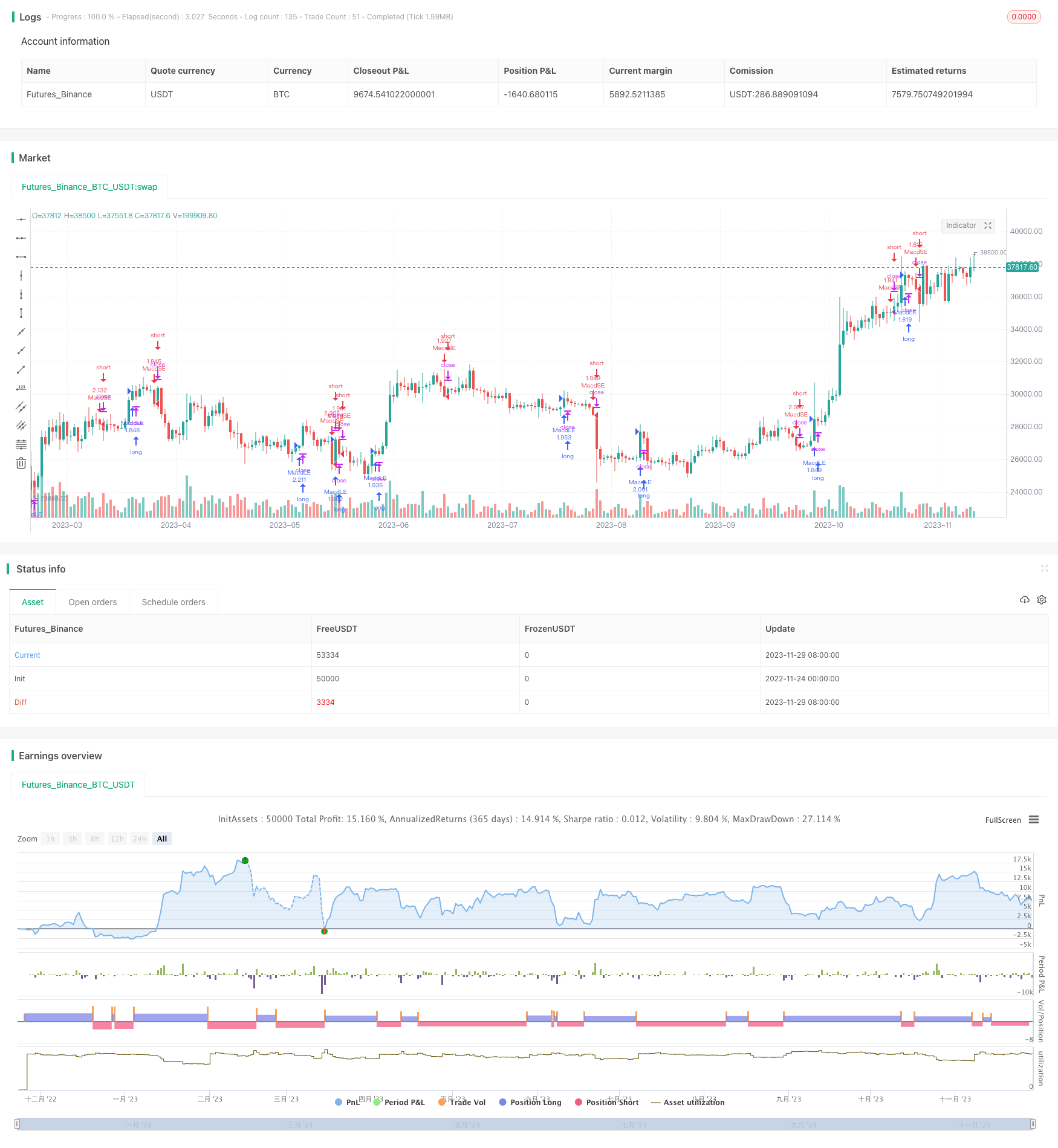
双均线交易策略通过计算不同周期的指数移动平均线,形成快线和慢线,并观察它们的金叉和死叉形态来产生交易信号。当快线从下方上穿慢线时,做多;当快线从上方下穿慢线时,做空。该策略捕捉了均线的趋势反转点,是一种较为常见的趋势跟踪策略。
策略原理
双均线交易策略的核心指标是计算快线和慢线。快线指短周期的指数移动平均线,默认参数为12日线;慢线指长周期的指数移动平均线,默认参数为26日线。指数移动平均线的计算公式为:
EMA(t) = (C(t) - EMA(t-1)) * SF + EMA(t-1)
其中,C(t)为当日收盘价,SF为smoothing factor 平滑因子。指数移动平均线与普通算术移动平均线的区别在于,指数移动平均线赋予了最近数据更大的权重,可以更快速地响应价格变化。
双均线策略的交易规则为:
- 当快线从下方上穿慢线时,即golden cross金叉形成,做多入场;
- 当快线从上方下穿慢线时,即dead cross死叉形成,做空入场;
- 快线和慢线发生背离时,平仓离场。
通过capture监控均线的交叉形态,及时反应市场供需关系和趋势的变化,实现盈利。
优势分析
双均线交易策略作为一种较为成熟的技术指标策略,具有以下优势:
- 思路清晰,易于理解和实现;
- 对市场供需关系的判断准确,胜率较高;
- 有效过滤市场噪音,捕捉主要趋势;
- 可在不同市场和时间框架下应用;
- 可与其他技术指标组合,丰富策略;
- 资金利用率高,符合大资金需求。
风险分析
双均线交易策略也存在一定的缺陷和风险:
- 无法应对剧烈行情,如快速熊市;
- 容易产生假信号和频繁小幅震荡带来密集交易;
- 需优化参数以适应不同品种和时间周期;
- 无法判断趋势反转的合理位置。
针对以上风险,可通过调整均线周期参数、引入附加过滤器等方法进行优化,确保策略更稳健。
优化方向
双均线交易策略可从以下几个方面进行优化:
- 引入MACD指标判断强弱趋势,避免弱势震荡行情的错误交易;
- 增加交易 volumes 作为确认指标,避免趋势反转的假突破;
- 结合其它如布林线、K线等技术指标,设定更精确的入场退场条件;
- 利用机器学习方法如LSTM自动优化均线参数,实现更好的市场适应性。
总结
双均线交易策略通过捕捉均线的金叉与死叉交易机会,判断价格趋势反转点,实现稳定盈利。该策略优势在于简洁清晰、资金效率高,是量化入门的首选策略。但也存在一定缺陷如产生假信号等,须引入更多指标进行优化,使其能更好地适应特定品种和交易环境。整体而言,双均线交易策略是一个非常实用的技术指标策略。
||
Overview
The dual moving average trading strategy generates trading signals by calculating exponential moving averages (EMAs) of different timeframes to form a fast EMA and slow EMA, and observing their golden crosses and death crosses. It goes long when the fast EMA crosses above the slow EMA, and goes short when the fast EMA crosses below the slow EMA. This strategy captures the trend reversal points of the moving averages and is a commonly used trend following strategy.
Strategy Logic
The core indicators of the dual moving average strategy are the fast EMA and slow EMA. The fast EMA has a default parameter of 12 days, while the slow EMA has a default parameter of 26 days. The formula for exponential moving average is:
EMA(t) = (C(t) - EMA(t-1)) x SF + EMA(t-1)
Where C(t) is today's closing price, and SF is the smoothing factor. Different from simple moving average, EMA assigns more weight to the recent data and thus responds faster to price changes.
The trading rules are:
-
Enter long positions on golden cross of fast EMA crossing above slow EMA from below.
-
Enter short positions on death cross of fast EMA crossing below slow EMA from above.
-
Exit positions on divergence of the EMAs.
By capturing the crossover patterns of the EMAs, it can reflect the market trends and increase profitability.
Advantages
As a mature technical indicator strategy, the dual moving average strategy has the following strengths:
-
Its logic is clear and easy to understand and implement.
-
It gives highly accurate judgement on market supply and demand and thus has relatively high win rate.
-
It effectively filters market noise and captures main trends.
-
It can be applied across different instruments and timeframes.
-
It can be combined with other indicators for strategy enrichment.
-
It has a high capital utilization efficiency for large capital trading.
Risk Analysis
There are also certain limitations of the strategy:
-
It fails to react to intense market moves like sharp bear market selloffs.
-
It tends to generate frequent false signals and whipsaws in sideways rangebound markets.
-
Its parameters need optimization across different markets and timeframes.
-
It cannot determine appropriate reversal levels of the trend.
The risks can be mitigated by adjusting EMA periods, adding supplementary filters etc. to make the strategy more robust.
Enhancement Opportunities
The dual moving average strategy can be improved from the following aspects:
-
Incorporate MACD indicator to judge trend strength and avoid wrong trades.
-
Add trading volumes to confirm true breakout signals.
-
Combine with Bollinger Bands, candlestick patterns for more precise entry and exit rules.
-
Utilize machine learning approaches like LSTM to auto optimize parameters for better adaptiveness.
Conclusion
The dual moving average trading strategy captures trading opportunities from EMA golden crosses and death crosses to determine trend reversal points for steady profits. With the advantages of simplicity, capital efficiency and ease of implementation, it is a preferred choice for algorithmic trading beginners. But it also has certain flaws like generating false signals. More indicators should be introduced to optimize it for specific markets and environments. Overall speaking, it is a very practical and useful technical indicator strategy.
[/trans]
Strategy Arguments
| Argument | Default | Description |
|---|---|---|
| v_input_1 | 12 | fastLength |
| v_input_2 | 26 | slowlength |
| v_input_3 | 9 | MACDLength |
| v_input_string_1 | Compound Equity | (?R & DD Table)Mode |
| v_input_int_1 | 2 | Return Precision |
| v_input_color_1 | #D4D4D4 | Headers Color |
| v_input_color_2 | black | Headers Text Color |
| v_input_color_3 | green | Positive Color |
| v_input_color_4 | red | Negative Color |
| v_input_color_5 | #DDDDDD | Zero Color |
| v_input_color_6 | white | Cell Text Color |
Source (PineScript)
/*backtest
start: 2022-11-24 00:00:00
end: 2023-11-30 00:00:00
period: 1d
basePeriod: 1h
exchanges: [{"eid":"Futures_Binance","currency":"BTC_USDT"}]
*/

// This source code is subject to the terms of the Mozilla Public License 2.0 at https://mozilla.org/MPL/2.0/
// © antondmt

//@version=5
strategy("Returns & Drawdowns Table", "R & DD", true, calc_on_every_tick = false, default_qty_type = strategy.percent_of_equity, default_qty_value = 100, process_orders_on_close = true)
i_eq_to_dd =            input.string("Compound Equity", "Mode", ["Simple Equity", "Compound Equity", "Drawdown"], group = "R & DD Table")
i_precision =           input.int(2, "Return Precision", group = "R & DD Table")
i_headers_col =         input.color(#D4D4D4, "Headers Color", group = "R & DD Table")
i_headers_text_col =    input.color(color.black, "Headers Text Color", group = "R & DD Table")
i_pos_col =             input.color(color.green, "Positive Color", group = "R & DD Table")
i_neg_col =             input.color(color.red, "Negative Color", group = "R & DD Table")
i_zero_col =            input.color(#DDDDDD, "Zero Color", group = "R & DD Table")
i_cell_text_col =       input.color(color.white, "Cell Text Color", group = "R & DD Table")

// TIME {
var month_times = array.new_int(0)                                                              // Array of all month times
new_month = month(time) != month(time[1])
if(new_month or barstate.isfirst)
    array.push(month_times, time)

var year_times = array.new_int(0)
new_year = year(time) != year(time[1])
if (new_year or barstate.isfirst)
    array.push(year_times, time)
//}

// SIMPLE EQUITY CALCULATIONS {
// Simple equity is strictly calculated from start to end of each month/year equity. There is no compound
var monthly_simp_pnls = array.new_float(0)                                                      // Array of all monthly profits and losses
var yearly_simp_pnls = array.new_float(0)

if(i_eq_to_dd == "Simple Equity")
    var initial_monthly_equity = strategy.equity                                                // Starting equity for each month
    cur_month_pnl = nz((strategy.equity - initial_monthly_equity) / initial_monthly_equity)     // Current month's equity change
    if(new_month or barstate.isfirst)
        initial_monthly_equity := strategy.equity
        array.push(monthly_simp_pnls, cur_month_pnl)
    else
        array.set(monthly_simp_pnls, array.size(monthly_simp_pnls) - 1, cur_month_pnl)

    var initial_yearly_equity = strategy.equity
    cur_year_pnl = nz((strategy.equity - initial_yearly_equity) / initial_yearly_equity)
    if (new_year or barstate.isfirst)
        initial_yearly_equity := strategy.equity
        array.push(yearly_simp_pnls, cur_year_pnl)
    else
        array.set(yearly_simp_pnls, array.size(yearly_simp_pnls) - 1, cur_year_pnl)
// }

// COMPOUND EQUITY CALCULATIONS {
// Compound equity is strictly calculated based on equity state from the beginning of time until the end of each month/year equity. It shows the exact equity movement through time
var monthly_comp_pnls = array.new_float(0)                                                      // Array of all monthly profits and losses
var yearly_comp_pnls = array.new_float(0)

if(i_eq_to_dd == "Compound Equity")
    var initial_equity = strategy.equity
    cur_month_pnl = nz((strategy.equity - initial_equity) / initial_equity)                     // Current month's equity change
    if(new_month or barstate.isfirst)
        array.push(monthly_comp_pnls, cur_month_pnl)
    else
        array.set(monthly_comp_pnls, array.size(monthly_comp_pnls) - 1, cur_month_pnl)

    cur_year_pnl = nz((strategy.equity - initial_equity) / initial_equity)
    if (new_year or barstate.isfirst)
        array.push(yearly_comp_pnls, cur_year_pnl)
    else
        array.set(yearly_comp_pnls, array.size(yearly_comp_pnls) - 1, cur_year_pnl)
// }

// DRAWDOWN CALCULATIONS {
// Drawdowns are calculated from highest equity to lowest trough for the month/year
var monthly_dds = array.new_float(0)                                                            // Array of all monthly drawdowns
var yearly_dds = array.new_float(0)

if (i_eq_to_dd == "Drawdown")
    total_equity = strategy.equity - strategy.openprofit

    var cur_month_dd = 0.0
    var m_ATH = total_equity                                                                    // Monthly All-Time-High (ATH). It is reset each month
    m_ATH := math.max(total_equity, nz(m_ATH[1]))
    m_drawdown = -math.abs(total_equity / m_ATH * 100 - 100) / 100                              // Drawdown at current bar
    if(m_drawdown < cur_month_dd)
        cur_month_dd := m_drawdown
    if(new_month or barstate.isfirst)
        cur_month_dd := 0.0
        m_ATH := strategy.equity - strategy.openprofit
        array.push(monthly_dds, 0)
    else
        array.set(monthly_dds, array.size(monthly_dds) - 1, cur_month_dd)

    var cur_year_dd = 0.0
    var y_ATH = total_equity
    y_ATH := math.max(total_equity, nz(y_ATH[1]))
    y_drawdown = -math.abs(total_equity / y_ATH * 100 - 100) / 100
    if(y_drawdown < cur_year_dd)
        cur_year_dd := y_drawdown
    if (new_year or barstate.isfirst)
        cur_year_dd := 0.0
        y_ATH := strategy.equity - strategy.openprofit
        array.push(yearly_dds, 0)
    else
        array.set(yearly_dds, array.size(yearly_dds) - 1, cur_year_dd)
// }

// TABLE LOGIC {
var main_table = table(na)
table.clear(main_table, 0, 0, 13, new_year ? array.size(year_times) - 1 : array.size(year_times))
main_table := table.new(position.bottom_right, columns = 14, rows = array.size(year_times) + 1, border_width = 1)

t_set_headers() =>                                                                              // Sets time headers of the table
    // Set month headers
    table.cell(main_table, 0,  0, "",     text_color = i_headers_text_col, bgcolor = i_headers_col)
    table.cell(main_table, 1,  0, "Jan",  text_color = i_headers_text_col, bgcolor = i_headers_col)
    table.cell(main_table, 2,  0, "Feb",  text_color = i_headers_text_col, bgcolor = i_headers_col)
    table.cell(main_table, 3,  0, "Mar",  text_color = i_headers_text_col, bgcolor = i_headers_col)
    table.cell(main_table, 4,  0, "Apr",  text_color = i_headers_text_col, bgcolor = i_headers_col)
    table.cell(main_table, 5,  0, "May",  text_color = i_headers_text_col, bgcolor = i_headers_col)
    table.cell(main_table, 6,  0, "Jun",  text_color = i_headers_text_col, bgcolor = i_headers_col)
    table.cell(main_table, 7,  0, "Jul",  text_color = i_headers_text_col, bgcolor = i_headers_col)
    table.cell(main_table, 8,  0, "Aug",  text_color = i_headers_text_col, bgcolor = i_headers_col)
    table.cell(main_table, 9,  0, "Sep",  text_color = i_headers_text_col, bgcolor = i_headers_col)
    table.cell(main_table, 10, 0, "Oct",  text_color = i_headers_text_col, bgcolor = i_headers_col)
    table.cell(main_table, 11, 0, "Nov",  text_color = i_headers_text_col, bgcolor = i_headers_col)
    table.cell(main_table, 12, 0, "Dec",  text_color = i_headers_text_col, bgcolor = i_headers_col)
    table.cell(main_table, 13, 0, str.tostring(i_eq_to_dd), text_color = i_headers_text_col, bgcolor = i_headers_col)

    // Set year headers
    for i = 0 to array.size(year_times) - 1
        table.cell(main_table, 0,  i + 1, str.tostring(year(array.get(year_times, i))), text_color = i_headers_text_col, bgcolor = i_headers_col)

t_set_months() =>                                                                               // Sets inner monthly data of the table
    display_array = switch i_eq_to_dd
        "Simple Equity" => monthly_simp_pnls
        "Compound Equity" => monthly_comp_pnls
        => monthly_dds
    for i = 0 to array.size(month_times) - 1
        m_row = year(array.get(month_times, i)) - year(array.get(year_times, 0)) + 1
        m_col = month(array.get(month_times, i))
        m_color = array.get(display_array, i) == 0 ? color.new(i_zero_col, transp = 30) : array.get(display_array, i) > 0 ? color.new(i_pos_col, transp = 30) : color.new(i_neg_col, transp = 30)
        table.cell(main_table, m_col, m_row, str.tostring(math.round(array.get(display_array, i) * 100, i_precision)), bgcolor = m_color, text_color = i_cell_text_col)

t_set_years() =>                                                                                // Sets inner yearly data of the table
    display_array = switch i_eq_to_dd
        "Simple Equity" => yearly_simp_pnls
        "Compound Equity" => yearly_comp_pnls
        => yearly_dds
    for i = 0 to array.size(year_times) - 1
        y_color = array.get(display_array, i) == 0 ? color.new(i_zero_col, transp = 30) : array.get(display_array, i) > 0 ? color.new(i_pos_col, transp = 20) : color.new(i_neg_col, transp = 20)
        table.cell(main_table, 13, i + 1, str.tostring(math.round(array.get(display_array, i) * 100, i_precision)), bgcolor = y_color, text_color = i_cell_text_col)

t_set_headers()
t_set_months()
t_set_years()
// }

// PLACE YOUR STRATEGY CODE HERE {
// This is a sample code of a working strategy to show the table in action
fastLength = input(12)
slowlength = input(26)
MACDLength = input(9)
MACD = ta.ema(close, fastLength) - ta.ema(close, slowlength)
aMACD = ta.ema(MACD, MACDLength)
delta = MACD - aMACD
if (ta.crossover(delta, 0))
	strategy.entry("MacdLE", strategy.long, comment = "MacdLE")
if (ta.crossunder(delta, 0))
	strategy.entry("MacdSE", strategy.short, comment = "MacdSE")
// }
Detail
https://www.fmz.com/strategy/433919
Last Modified
2023-12-01 14:36:33