strategies/多时间轴均线系统交易策略Multi-Timeframe-Moving-Average-System-Trading-Strategy.md

Name

多时间轴均线系统交易策略Multi-Timeframe-Moving-Average-System-Trading-Strategy

Author

ChaoZhang

Strategy Description

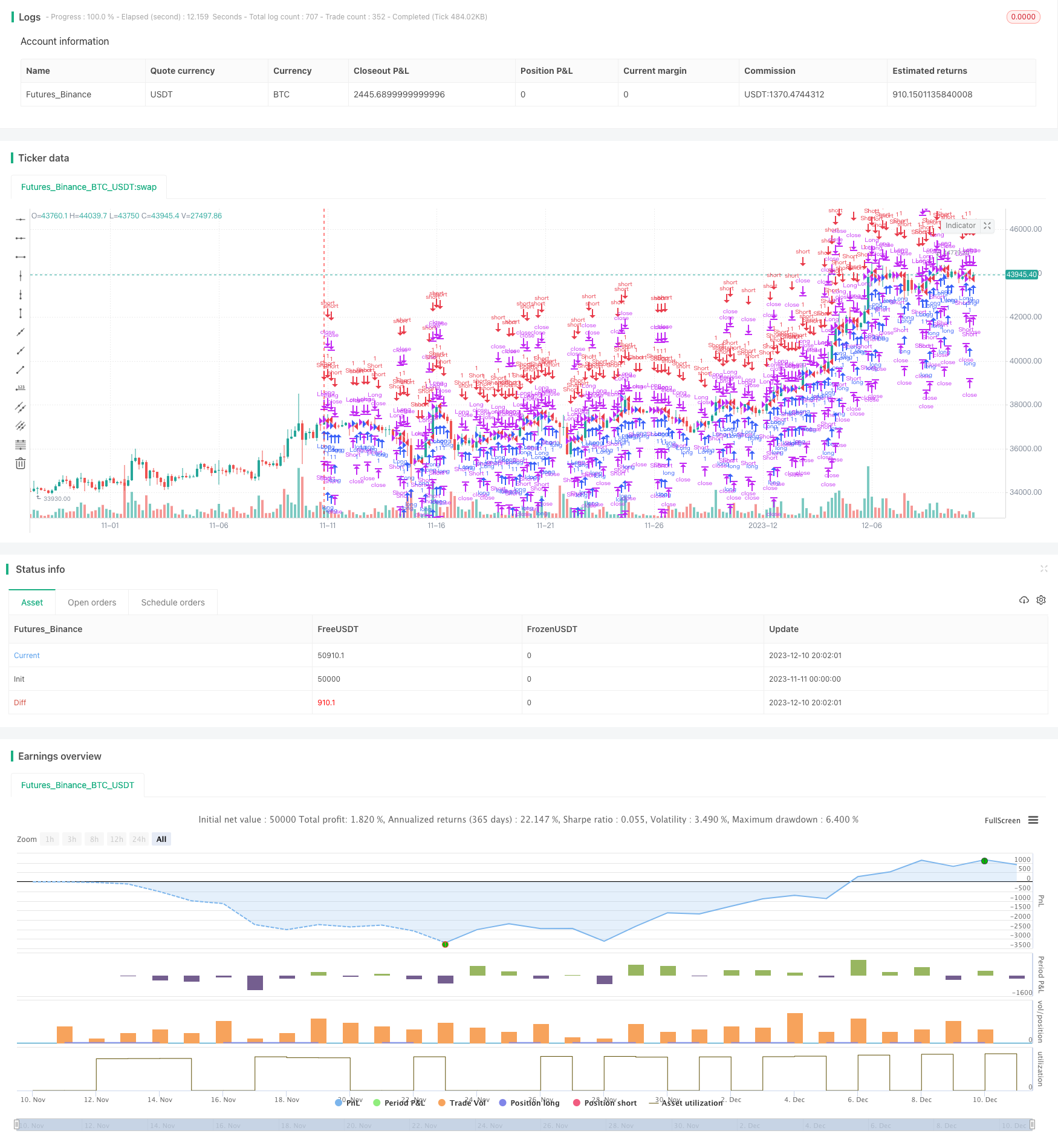[trans]

概述

本策略采用多重时间轴的均线系统,结合RSI指标等多种技术指标,实现多空自动切换。策略名称为“Multi-Timeframe Moving Average System Trading Strategy”,主要思想是通过比较不同时间段内价格的趋势判断,实现更加可靠的交易信号产生。

策略原理

该策略的核心指标为均线系统。策略使用 JMA、TEMA、DEMA 等多种均线指标在 15分钟、30分钟、60分钟等不同周期内计算价格趋势。例如 15周期内使用 JMA 计算出来的均线走势作为该周期内的价格趋势判断。然后策略将不同周期内的价格走势进行比较,判断长线与短线之间是否存在背离。如果存在显著的背离信号,则产生交易信号。此外,策略还结合 RSI、波浪指标等辅助判断,确保交易信号的可靠性。

具体来说,策略中的 trend、trend2 和 trend3 变量分别代表 15分钟、30分钟和 60 分钟的价格趋势。如果 15分钟价格反转,而 30分钟和 60 分钟还没有反转,那么就判断为短线和长线之间存在背离,则产生交易信号。如果所有周期趋势一致,则不产生交易信号。

这样通过比较多个周期之间的关系,过滤掉一些假信号,产生更加可靠的交易信号,这是该策略的核心思路。

优势分析

该策略主要具有以下优势:

1. 使用多时间轴分析,提高信号的可靠性,过滤假信号;
2. 结合多种指标进行综合判断,避免单一指标带来的问题;
3. 自动实现多空头切换,无需人工干预,降低操作难度。

风险分析

该策略也存在一些风险:

1. 多时间轴分析,将增加交易时点的不确定性,可能错过最佳进场时机;
2. 同时结合多种指标,指标参数设置不当可能会产生交易信号质量下降的问题;
3. 自动切换多空头存在过优化风险,实盘效果可能弱于回测。

针对上述风险,我们可以采取以下措施加以缓解:

1. 调整时间轴参数,确保及时获知短线信号以 vez 进场;
2. 通过大量数据回测,不断优化指标参数;
3. 在实盘中适当干预,避免自动系统盲目交易。

优化方向

该策略还存在进一步优化的空间:

1. 可以引入机器学习算法,通过模型训练自动优化多指标参数;
2. 可以增加自适应滑点设置,根据市场波动程度调整滑点大小,提高实盘效果;
3. 可以引入量价确认机制,避免趋势快速反转带来的损失。

总结

本策略通过比较多时间轴价格走势判断长短线关系,结合多种指标综合分析产生交易信号,实现自动多空头切换,回测效果较好。我们也发现该策略存在一定改进空间,未来通过引入机器学习、自适应滑点、量价确认等方法进行优化,可望进一步提高策略的实盘效果。

||

Overview

This strategy adopts a multi-timeframe moving average system, combined with RSI and other technical indicators, to achieve automatic switching between long and short positions. The strategy name is “Multi-Timeframe Moving Average System Trading Strategy”. The main idea is to generate more reliable trading signals by comparing price trends over different time periods.

Principles

The core indicators of this strategy are the moving average system. The strategy uses multiple moving average indicators such as JMA, TEMA, DEMA to calculate price trends over different periods like 15min, 30min, 60min. For example, the MA trend calculated by JMA in the 15min timeframe represents the price trend judgement within that timeframe. Then the strategy compares price trends between different timeframes to identify divergences between longer and shorter trends. If significant divergences are detected, trading signals will be generated. In addition, the strategy also incorporates other indicators like RSI and Wave Trend to ensure reliability of trading signals.

Specifically, the trend, trend2 and trend3 variables in the strategy represent price trends of the 15min, 30min and 60min timeframes respectively. If there is a 15min price reversal, while 30min and 60min has not reversed yet, it is judged as a divergence between shorter and longer trends, hence producing a trading signal. No signals will be generated if trends of all timeframes are consistent.

By comparing relationships between multiple timeframes and filtering out some false signals, more reliable trading signals can be generated – this is the core idea of the strategy.

Advantage Analysis

The main advantages of this strategy are:

1. Improved signal reliability through multi-timeframe analysis and filtering of false signals;
2. Avoiding issues with single indicators by combining multiple indicators for comprehensive judgements;
3. Automatic switching between long and short positions without manual interventions, reducing operational difficulty.

Risk Analysis

Some risks also exist with this strategy:

1. Multi-timeframe analysis introduces uncertainty around trade entry timing which may cause missing of best entry prices;
2. Inappropriate parameter settings when combining multiple indicators could lead to deteriorating trading signal quality;
3. Automatic position switching risks over-optimization and weaker real-trading performance versus backtests.

We can take the following measures to mitigate the above risks:

1. Fine-tune timeframe parameters to ensure capturing short-term signals for timely entry;
2. Extensive backtesting to continuously optimize indicator parameters;
3. Reasonable interventions in real trading to prevent blind trading by automated systems.

Optimization Directions

There is room for further optimization of this strategy:

1. Introduce machine learning algorithms to auto-optimize parameters across multiple indicators through model training;
2. Add adaptive slippage settings based on market volatility levels to improve real-trading performance;
3. Incorporate price-volume confirmation mechanisms to avoid losses from rapid trend reversals.

Conclusion

This strategy compares multi-timeframe price trends to identify longer versus shorter term relationships, and generates trading signals through analyzing multiple indicators – achieving automatic switching between longs and shorts with good backtest results. We also identified some areas of improvement via methods like machine learning, adaptive slippage and volume confirmation to further enhance real-trading performance.

[/trans]

Strategy Arguments

Argument	Default	Description
v_input_1	1.5	Multiplier

Source (PineScript)

/*backtest
start: 2023-11-11 00:00:00
end: 2023-12-11 00:00:00
period: 4h
basePeriod: 15m
exchanges: [{"eid":"Futures_Binance","currency":"BTC_USDT"}]
*/

//@version=2
strategy("Drexel Strategy", overlay=true )
Length1=7
Length2=9
Multiplier=input(1.5,"Multiplier")
jma(src,length) =>
    beta = 0.45*(length-1)/(0.45*(length-1)+2)
    alpha = beta
    tmp0 = (1-alpha)*src + alpha*nz(tmp0[1])
    tmp1 = (src - tmp0[0])*(1-beta) + beta*nz(tmp1[1])
    tmp2 = tmp0[0] + tmp1[0]
    tmp3 = (tmp2[0] - nz(tmp4[1]))*((1-alpha)*(1-alpha)) + (alpha*alpha)*nz(tmp3[1])
    tmp4 = nz(tmp4[1]) + tmp3[0]
    JMA = tmp4
    JMA
rsx(src,length) =>
    f90_ = (nz(f90_[1]) == 0.0) ? 1.0 : (nz(f88[1]) <= nz(f90_[1])) ? nz(f88[1])+1 : nz(f90_[1])+1
    f88 = (nz(f90_[1]) == 0.0) and (length-1 >= 5) ? length-1.0 : 5.0 
    f8 =  100.0*(src) 
    f18 = 3.0 / (length + 2.0) 
    f20 = 1.0 - f18 
    f10 = nz(f8[1])
    v8 = f8 - f10 
    f28 = f20 * nz(f28[1]) + f18 * v8 
    f30 = f18 * f28 + f20 * nz(f30[1])
    vC = f28 * 1.5 - f30 * 0.5 
    f38 = f20 * nz(f38[1]) + f18 * vC 
    f40 = f18 * f38 + f20 * nz(f40[1])
    v10 = f38 * 1.5 - f40 * 0.5 
    f48 = f20 * nz(f48[1]) + f18 * v10 
    f50 = f18 * f48 + f20 * nz(f50[1])
    v14 = f48 * 1.5 - f50 * 0.5 
    f58 = f20 * nz(f58[1]) + f18 * abs(v8) 
    f60 = f18 * f58 + f20 * nz(f60[1])
    v18 = f58 * 1.5 - f60 * 0.5
    f68 = f20 * nz(f68[1]) + f18 * v18 
    f70 = f18 * f68 + f20 * nz(f70[1])
    v1C = f68 * 1.5 - f70 * 0.5 
    f78 = f20 * nz(f78[1]) + f18 * v1C 
    f80 = f18 * f78 + f20 * nz(f80[1])
    v20 = f78 * 1.5 - f80 * 0.5
    f0 = ((f88 >= f90_) and (f8 != f10)) ? 1.0  : 0.0
    f90 = ((f88 == f90_) and (f0 == 0.0))  ? 0.0  : f90_
    v4_ = ((f88 < f90) and (v20 > 0.0000000001)) ? (v14 / v20 + 1.0) * 50.0 : 50.0
    rsx = ((v4_ > 100.0) ? 100.0 : (v4_ < 0.0) ? 0.0 : v4_)-50
    rsx
xPrice=open
emaA = ema(xPrice, Length2)  
Xprice = rsx(open,14)
XPrice = high, xprice = low
xe1 = jma(xPrice, Length1)
xe11 = jma(Xprice[1],Length1)
xe111 = jma(XPrice[1],Length1)
xe1111=jma(xprice[1],Length1)
xe2 = jma(xe1, Length1)
xe21 = jma(xe111, Length1)
xe3 = jma(xe2, Length1)
xe31 = jma(xe1111,Length2)
xe3a = jma(xe2,Length1)
xe4 = jma(xe3, Length1)
xe5 = jma(xe4, Length1)
xe6 = jma(xe5, Length1)
b = 0.7
c1 = -b*b*b
c2 = 3*b*b+3*b*b*b
c3 = -6*b*b-3*b-3*b*b*b
c3a = nz(c3a[1])
c4 = 1+3*b+b*b*b+3*b*b
TEMA = c1 * xe6 + c2 * xe5 + c3 * xe4 + c4 * xe3
DEMA = 2 * emaA - ema(emaA, Length2)
Length(mod)=>(mod*c3a)+Length2
Trend1=TEMA/DEMA
a=rsx(open,Length(2))
b1=rsx(open,Length(3))
c=rsx(open,Length(5))
d=rsx(open,Length(8))
e=rsx(open,Length(13))
f=rsx(open,Length(21))
g=rsx(open,Length(34))
h=rsx(open,Length(55))
i=rsx(open,Length(89))
j=rsx(open,Length(144))
trend1 = (((a-b1)+(c-d)+(e-f)+(g-h)+(i-j))/10)
trend = trend1>0?avg(a,b,c4,c2):trend1==0?XPrice:avg(rsx(open,24),jma(open,24),rsx(jma(open,24),24))
trend2 = trend1>0?avg(d,e,c2,c1):trend1==0?XPrice:avg(rsx(open,48),jma(open,48),rsx(jma(open,48),48))
trend3 = trend1>0?avg(d,e,c2,c1):trend1==0?xprice:avg(rsx(open,96),jma(open,96),rsx(jma(open,96),96))
bc=request.security(syminfo.tickerid,'15',trend)
bc1=request.security(syminfo.tickerid,'15',trend2)
bc2=request.security(syminfo.tickerid,'15',trend3)
bd=request.security(syminfo.tickerid,'30',trend)
bd1=request.security(syminfo.tickerid,'30',trend2)
bd2=request.security(syminfo.tickerid,'30',trend3)
be=request.security(syminfo.tickerid,'60',trend)
be1=request.security(syminfo.tickerid,'60',trend2)
be2=request.security(syminfo.tickerid,'60',trend3)
bf=request.security(syminfo.tickerid,'120',trend)
bf1=request.security(syminfo.tickerid,'120',trend2)
bf2=request.security(syminfo.tickerid,'120',trend3)
bg=request.security(syminfo.tickerid,'240',trend)
bg1=request.security(syminfo.tickerid,'240',trend2)
bg2=request.security(syminfo.tickerid,'240',trend3)
bh=request.security(syminfo.tickerid,'D',trend)
bh1=request.security(syminfo.tickerid,'D',trend2)
bh2=request.security(syminfo.tickerid,'D',trend3)
Trend=((bc-bc1)+(bd-bd1)+(be-be1)+(bf-bf1)+(bg-bg1)+(bh))
Trend11=((bc-bc1)+(bd-bd1)+(be-be1)+(bf-bf1)+(bg-bg1)+(bh1))
Trend33 = max(min(min(min(bc2,bd2),min(be2,bf2)),bg2),bh2)
AverageTrend=sma(Trend1,1000)
StdDev=Multiplier*stdev(Trend1,1000)
TopBand=AverageTrend+StdDev
BotBand=AverageTrend-StdDev
ap=open
n1=10
n2=21
esa1 = jma(ap, n1)
d1 = jma(abs(ap - esa1), n1)
x1 = trend3==Trend33
y1 = trend2==Trend11 
ci = (ap - esa1) / (0.015 * d1)
tci = jma(ci, n2)
wt1=tci
wt2=sma(wt1,4)
fast=jma(open,5)
slow=jma(open,13)
macd=fast-slow
signal=sma(macd,4)
WaveTrend1=wt1-wt2
JMACD1=macd-signal
rsi = (((rsi(open,6))-50)*3)
g1=rsi>Trend1 and WaveTrend1>Trend1 and JMACD1>Trend1
h1=g1?tci*c3a:nz(h[1])
strategy.entry("Long",true,when=x1)
strategy.close("Long",y1)
strategy.entry("Short",false,when=y1)
strategy.close("Short",x1)

Detail

https://www.fmz.com/strategy/435138

Last Modified

2023-12-12 16:07:18