strategies/动量指标决策交易策略Momentum-Indicator-Decision-Trading-Strategy.md

Name

动量指标决策交易策略Momentum-Indicator-Decision-Trading-Strategy

Author

ChaoZhang

Strategy Description

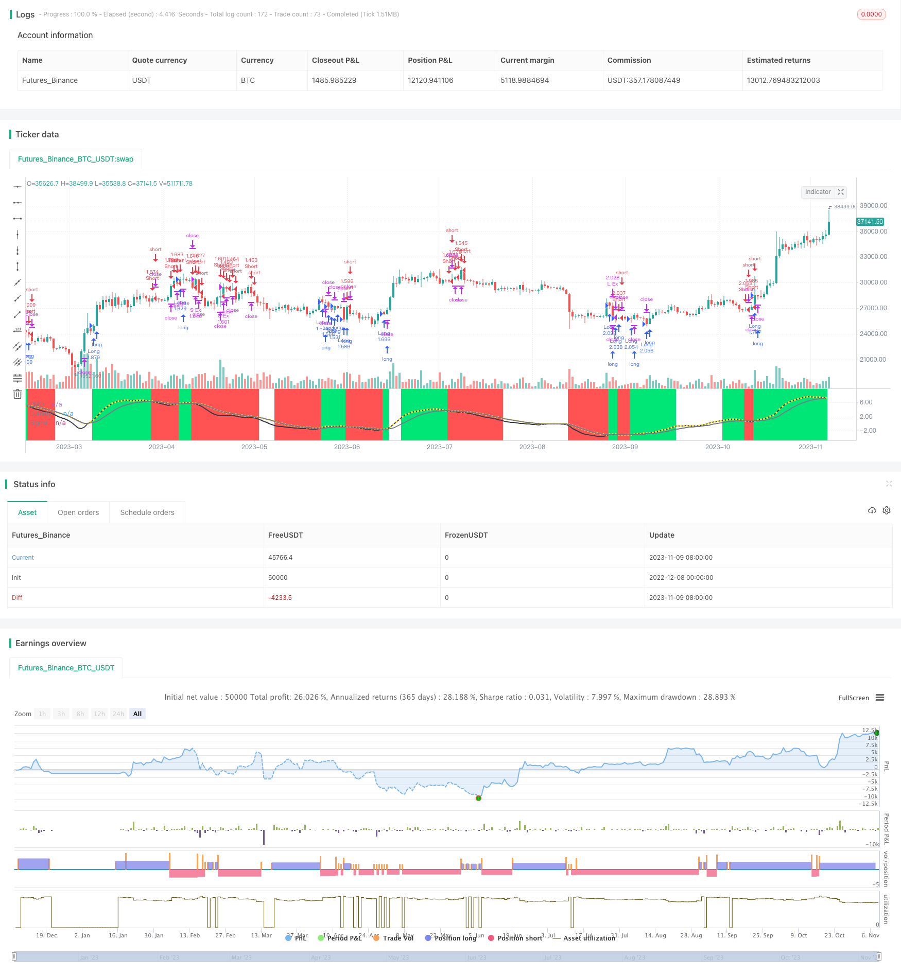
[trans]

概述

动量指标决策交易策略是一种趋势跟踪策略。它使用双指数移动平均线构建动量指标,然后结合价格的变化率指标来产生交易信号。当动量指标上涨时,产生做多信号;当动量指标下跌时,产生做空信号。该策略适用于追踪市场中期趋势的交易者。

策略原理

该策略使用双指数移动平均线指标Decision Point oscillator来测量动量。首先计算价格的每日变化率,然后使用长度为31天和20天的双指数移动平均线分别平滑价格变化率,最后用9天的平滑移动平均线来发出交易信号。当快线高于慢线时为多头市场,当快线低于慢线时为空头市场。

该策略还引入价格变化率指标,以避免在盘整市场中产生错误信号。具体来说,是计算近30天价格的百分比变化率,通过其移动平均线来判断市场是否处于活跃状态。只有在市场活跃时,才会发出交易信号。

优势分析

该策略结合动量指标和价格变化率指标,可以有效识别中期趋势,避免在震荡行情中频繁交易。相比简单跟踪移动平均线等趋势策略,它可以大幅度降低错误交易的概率。此外,风险控制方面设置了止损点,可以及时止损,有效控制单笔损失。

风险分析

该策略主要 BASE在中长线趋势交易,无法捕捉短期价格波动。当出现剧烈行情时,止损点可能会被突破,导致较大亏损。此外,参数设置不当也会对策略产生影响。例如双指数移动平均线参数设置过短,会增加错误交易的概率。

要防范风险,可以适当调整止损点,扩大止损幅度。也可以在剧烈行情来临时,暂时关闭策略,避免止损被突破的概率。参数调整方面,应该进行详细的回测,选择最优参数。

优化方向

该策略可以从以下几个方向进行优化:

1. 增加其他过滤指标,如波动率指标,可以避免行情剧烈波动期间的交易。

2. 增加机器学习模型,辅助判断趋势方向和力度,可以提高信号的准确性。

3. 尝试不同的动量指标,如相对强弱指标、Stochastic oscillator等,优化买卖时机。

4. 实盘运行过程中,结合最近期行情特点,动态调整参数,追求最优参数组合。

总结

动量指标决策交易策略整体来说是一种稳健的中长期趋势跟踪策略。它结合双指数移动平均线动量指标和价格变化率指标,可以有效识别趋势,避免错误交易。同时,设置止损点来控制风险。如果参数调整合理,回测效果良好,则适合中长线追求超额收益的投资者。当然,交易者仍需警惕行情剧烈波动给策略带来的冲击风险。

||

Overview

The Momentum Indicator Decision Trading Strategy is a trend following strategy. It builds a momentum indicator using double exponential moving average and combines it with price rate of change indicator to generate trading signals. When the momentum indicator goes up, it generates long signals. When the momentum indicator goes down, it generates short signals. This strategy suits traders who want to track mid-term trends in the market.

Strategy Principle

The strategy uses Decision Point oscillator based on double exponential moving average to measure momentum. First it calculates the daily price change rate, then uses 31-day and 20-day double exponential moving averages to smooth the price change rate separately. Finally it uses a 9-day smoothed moving average to issue trading signals. When the fast line is above the slow line, it indicates a bull market. When the fast line is below the slow line, it indicates a bear market.

The strategy also introduces a price rate of change indicator to avoid wrong signals in sideways markets. Specifically, it calculates the percentage price change over the past 30 days, and judges whether the market is active through its moving average. Trading signals are only issued when the market is active.

Advantage Analysis

The strategy combines momentum indicator and price rate of change indicator, which can effectively identify mid-term trends and avoid frequent trading in volatile markets. Compared to simple trend following strategies like moving average, it can greatly reduce the probability of wrong trades. In addition, risk is controlled by setting stop loss points to cut losses in time and effectively control per trade loss.

Risk Analysis

The strategy mainly relies on mid-long term trend trading, unable to capture short-term price fluctuations. When there is a sharp market movement, the stop loss point may be broken, leading to greater losses. In addition, inappropriate parameter settings can also affect the strategy. For example, if the double exponential moving average parameters are set too short, the probability of wrong trades will increase.

To prevent risks, stop loss points can be adjusted appropriately to expand stop loss range. When a sharp market movement happens, the strategy can be temporarily turned off to avoid the probability of stop loss being broken. For parameter tuning, detailed backtesting should be performed to select the optimal parameters.

Optimization Directions

The strategy can be optimized in the following aspects:

1. Add other filtering indicators like volatility indicator to avoid trading during periods of sharp market fluctuations.

2. Add machine learning models to assist judgment of trend direction and strength, which can improve signal accuracy.

3. Try different momentum indicators like Relative Strength Index, Stochastic oscillator to optimize entry and exit timing.

4. In live trading, dynamically adjust parameters combined with recent market conditions to pursue optimal parameter combination.

Conclusion

The Momentum Indicator Decision Trading Strategy is generally a steady mid-long term trend following strategy. It effectively identifies trends and avoids wrong trades by combining double exponential moving average momentum indicator and price rate of change indicator. Meanwhile, it controls risk by setting stop loss points. If parameters are tuned properly and backtest results are good, it suits mid-long term investors who pursue excess returns. Of course, traders still need to be aware of the risk brought by sharp market fluctuations to the strategy.

[/trans]

Strategy Arguments

Argument	Default	Description
v_input_1	2017	Backtest Start Year
v_input_2	true	Backtest Start Month
v_input_3	true	Backtest Start Day
v_input_4	2019	Backtest Stop Year
v_input_5	12	Backtest Stop Month
v_input_6	31	Backtest Stop Day
v_input_7_ohlc4	0	Source: ohlc4
v_input_8	31	First Smoothing
v_input_9	20	Second Smoothing
v_input_10	9	Signal Smoothing
v_input_11	true	Fill Region
v_input_12	30	roclength
v_input_13	7	pcntChange
v_input_14	2	Stop Loss %
v_input_15	5000	Take Profit %

Source (PineScript)

/*backtest
start: 2022-12-08 00:00:00
end: 2023-11-10 00:00:00
period: 1d
basePeriod: 1h
exchanges: [{"eid":"Futures_Binance","currency":"BTC_USDT"}]
*/

//@version=4
strategy("Decision BF", overlay=false, initial_capital=10000, default_qty_type=strategy.percent_of_equity, default_qty_value=100, commission_type=strategy.commission.percent, commission_value=0.075)

/////////////// Time Frame ///////////////
testStartYear = input(2017, "Backtest Start Year") 
testStartMonth = input(1, "Backtest Start Month")
testStartDay = input(1, "Backtest Start Day")
testPeriodStart = timestamp(testStartYear,testStartMonth,testStartDay, 0, 0)

testStopYear = input(2019, "Backtest Stop Year")
testStopMonth = input(12, "Backtest Stop Month")
testStopDay = input(31, "Backtest Stop Day")
testPeriodStop = timestamp(testStopYear,testStopMonth,testStopDay, 0, 0)

testPeriod() => true

/////////////// Decision ///////////////
src = input(ohlc4, title="Source")
length1 = input(31, title="First Smoothing")
length2 = input(20, title="Second Smoothing")
siglength = input(9, title="Signal Smoothing")
fr = input(true, title="Fill Region")

calc_csf(src, length) => 
	sm = 2.0 / length
	csf = 0.0
	csf := (src - nz(csf[1])) * sm + nz(csf[1])
	csf
i = (src / nz(src[1], src)) * 100
pmol2 = calc_csf(i - 100, length1)
pmol = calc_csf(10 * pmol2, length2)
pmols = ema(pmol, siglength)
d = pmol - pmols
duml = plot(fr ? (d > 0 ? pmol : pmols) : na, style=plot.style_circles, color=color.yellow, linewidth=0, title="DummyL")

hc = d > 0 ? d > d[1] ? color.lime : color.green : d < d[1] ? color.red : color.orange

///////////// Rate Of Change ///////////// 
source = close
roclength = input(30, minval=1)
pcntChange = input(7, minval=1)
roc = 100 * (source - source[roclength]) / source[roclength]
emaroc = ema(roc, roclength / 2)
isMoving() => emaroc > (pcntChange / 2) or emaroc < (0 - (pcntChange / 2))

/////////////// Strategy ///////////////
long = d > 0 and isMoving() 
short = d < 0 and isMoving() 

last_long = 0.0
last_short = 0.0
last_long := long ? time : nz(last_long[1])
last_short := short ? time : nz(last_short[1])

long_signal = crossover(last_long, last_short)
short_signal = crossover(last_short, last_long)

last_open_long_signal = 0.0
last_open_short_signal = 0.0
last_open_long_signal := long_signal ? open : nz(last_open_long_signal[1])
last_open_short_signal := short_signal ? open : nz(last_open_short_signal[1])

last_long_signal = 0.0
last_short_signal = 0.0
last_long_signal := long_signal ? time : nz(last_long_signal[1])
last_short_signal := short_signal ? time : nz(last_short_signal[1])

in_long_signal = last_long_signal > last_short_signal
in_short_signal = last_short_signal > last_long_signal

last_high = 0.0
last_low = 0.0
last_high := not in_long_signal ? na : in_long_signal and (na(last_high[1]) or high > nz(last_high[1])) ? high : nz(last_high[1])
last_low := not in_short_signal ? na : in_short_signal and (na(last_low[1]) or low < nz(last_low[1])) ? low : nz(last_low[1])

sl_inp = input(2.0, title='Stop Loss %') / 100
tp_inp = input(5000.0, title='Take Profit %') / 100
 
take_level_l = strategy.position_avg_price * (1 + tp_inp)
take_level_s = strategy.position_avg_price * (1 - tp_inp)

since_longEntry = barssince(last_open_long_signal != last_open_long_signal[1]) 
since_shortEntry = barssince(last_open_short_signal != last_open_short_signal[1])

slLong = in_long_signal ? strategy.position_avg_price * (1 - sl_inp) : na
slShort = strategy.position_avg_price * (1 + sl_inp)
long_sl = in_long_signal ? slLong : na
short_sl = in_short_signal ? slShort : na

/////////////// Execution ///////////////
if testPeriod()
    strategy.entry("Long",  strategy.long, when=long)
    strategy.entry("Short", strategy.short, when=short)
    strategy.exit("L Ex", "Long", stop=long_sl, limit=take_level_l, when=since_longEntry > 0)
    strategy.exit("S Ex", "Short", stop=short_sl, limit=take_level_s, when=since_shortEntry > 0)

/////////////// Plotting ///////////////
sigl = plot(false ? na : pmols, title="PMO Signal", color=color.gray, linewidth=2, title="Signal")
mdl = plot(false ? na : pmol, title="PMO", color=color.black, linewidth=2, title="PMO")
fill(duml, sigl, color.green, transp=20, title="PosFill")
fill(duml, mdl, color.red, transp=20, title="NegFill")
bgcolor(isMoving() ? long ? color.lime : short ? color.red : na : color.white, transp=70)
bgcolor(long_signal ? color.lime : short_signal ? color.red : na, transp=50)

Detail

https://www.fmz.com/strategy/435502

Last Modified

2023-12-15 15:31:52