strategies/动量跟踪自适应统计套利策略Momentum-Tracking-Adaptive-Statistical-Arbitrage-Strategy.md

Name

动量跟踪自适应统计套利策略Momentum-Tracking-Adaptive-Statistical-Arbitrage-Strategy

Author

ChaoZhang

Strategy Description

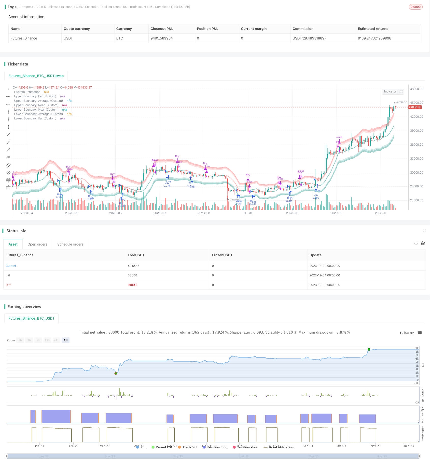[trans]

概述

该策略基于Nadaraya-Watson核回归方法构建了一个动态波动率包围带,通过跟踪价格与包围带的交叉情况,实现低买高卖的交易信号。策略具有数学分析基础,能够自适应市场变化。

策略原理

策略的核心是计算价格的动态包围带。首先,根据自定义的看回期,构建价格(收盘价、最高价、最低价)的Nadaraya-Watson核回归曲线,得到平滑化的价格估计。然后基于自定义的ATR长度计算ATR指标,结合近端因子和远端因子,得到上下包围带的范围。当价格从下包围带下方突破进入包围带,产生买入信号;当价格从上包围带上方突破离开包围带,产生卖出信号。该策略通过跟踪价格与波动率相关的统计属性,动态调整交易决策。

策略优势

1. 基于数学模型,参数可控,不容易产生过度优化
2. 自适应市场变化,利用价格与波动率的动态关系捕捉交易机会
3. 采用对数坐标,能够很好处理不同时间周期和波动幅度的品种
4. 可自定义参数调整策略的灵敏度

策略风险

1. 数学模型理论化,实盘表现可能不如预期
2. 关键参数选取需要经验,不当设置可能影响收益
3. 存在一定的滞后,可能错过部分交易机会
4. 大幅震荡市场中容易出现错误信号

主要通过优化参数,做好回测,了解影响因素,谨慎实盘来规避和减少这些风险。

策略优化方向

1. 进一步优化参数,找出最佳参数组合
2. 利用机器学习方法自动优选参数
3. 增加过滤条件,在特定市场环境下激活策略
4. 结合其他指标过滤误导信号
5. 尝试不同的数学模型算法

总结

该策略整合统计分析与技术指标分析,通过动态跟踪价格与波动率,实现低买高卖的交易信号。可根据市场和自身情况调整参数。整体来说,策略理论基础坚实,实际表现还有待进一步验证。需要谨慎看待,审慎实盘。

||

Overview

This strategy builds a dynamic volatility envelope based on the Nadaraya-Watson kernel regression method to generate trading signals of buying low and selling high by tracking the crossover situations between price and the envelope bands. With a mathematical analysis framework, the strategy can adapt itself to the market changes.

Strategy Logic

The core of the strategy is to calculate the dynamic envelope of the price. Firstly, by using a custom lookback window, it constructs the Nadaraya-Watson kernel regression curves of the price (close, high, low) to get a smoothed price estimation. Then it calculates the ATR based on a custom ATR length, and forms the upper and lower envelope bands with near and far factors. When the price breaks into the envelope from below, a buy signal is generated. When the price breaks out of the envelope from above, a sell signal is triggered. By tracking the dynamic relationship between price and volatility-related statistical properties, the strategy adjusts its trading decisions adaptively.

Advantages

1. Based on mathematical models with controllable parameters, less probability of overfitting.
2. Adaptive to market changes by leveraging dynamic relationship between price and volatility to catch trading opportunities.
3. Log scale works well with different timeframes and instruments with varying volatility magnitudes.
4. Customizable parameters to adjust strategy sensitivity.

Risks

1. Theoretical nature of mathematical models, may underperform in live trading.
2. Key parameters need expertise, improper settings may hurt profitability.
3. Lagging issue may cause missing some trading chances.
4. Vulnerable to whipsaws in highly volatile markets.

Proper optimization, sufficient backtest, understanding key factors and prudent position sizing in live trading could help mitigate these risks.

Improvement Directions

1. Further optimize parameters to find best combination.
2. Apply machine learning methods to auto-select optimal parameters.
3. Add filters to activate strategy in certain market environments.
4. Incorporate other indicators to filter misleading signals.
5. Try different mathematical model algorithms.

Conclusion

The strategy incorporates statistical analysis and technical indicators analysis to generate trading signals by dynamically tracking the relationship between price and volatility. The parameters can be adjusted based on market conditions and personal needs. Overall speaking, despite the solid theoretical foundation, its actual performance still needs further verification. One should treat it prudently and trade cautiously.
[/trans]

Strategy Arguments

Argument	Default	Description
v_input_int_1	8	(?Custom Settings)Lookback Window (Custom)
v_input_float_1	8	Relative Weighting (Custom)
v_input_int_2	25	Start Regression at Bar (Custom)
v_input_int_3	60	ATR Length (Custom)
v_input_float_2	1.5	Near ATR Factor (Custom)
v_input_float_3	2	Far ATR Factor (Custom)

Source (PineScript)

/*backtest
start: 2022-12-04 00:00:00
end: 2023-12-10 00:00:00
period: 1d
basePeriod: 1h
exchanges: [{"eid":"Futures_Binance","currency":"BTC_USDT"}]
*/

// © Julien_Eche
//@version=5

strategy("Nadaraya-Watson Envelope Strategy", overlay=true, pyramiding=1, default_qty_type=strategy.percent_of_equity, default_qty_value=20)

// Helper Functions
getEnvelopeBounds(_atr, _nearFactor, _farFactor, _envelope) => 
    _upperFar = _envelope + _farFactor*_atr
    _upperNear = _envelope + _nearFactor*_atr
    _lowerNear = _envelope - _nearFactor*_atr
    _lowerFar = _envelope - _farFactor*_atr
    _upperAvg = (_upperFar + _upperNear) / 2
    _lowerAvg = (_lowerFar + _lowerNear) / 2 
    [_upperNear, _upperFar, _upperAvg, _lowerNear, _lowerFar, _lowerAvg]

customATR(length, _high, _low, _close) =>
    trueRange = na(_high[1])? math.log(_high)-math.log(_low) : math.max(math.max(math.log(_high) - math.log(_low), math.abs(math.log(_high) - math.log(_close[1]))), math.abs(math.log(_low) - math.log(_close[1])))
    ta.rma(trueRange, length)

customKernel(x, h, alpha, x_0) =>
    sumWeights = 0.0
    sumXWeights = 0.0
    for i = 0 to h
        weight = math.pow(1 + (math.pow((x_0 - i), 2) / (2 * alpha * h * h)), -alpha)
        sumWeights := sumWeights + weight
        sumXWeights := sumXWeights + weight * x[i]
    sumXWeights / sumWeights

// Custom Settings
customLookbackWindow = input.int(8, 'Lookback Window (Custom)', group='Custom Settings')
customRelativeWeighting = input.float(8., 'Relative Weighting (Custom)', step=0.25, group='Custom Settings')
customStartRegressionBar = input.int(25, "Start Regression at Bar (Custom)", group='Custom Settings')

// Envelope Calculations
customEnvelopeClose = math.exp(customKernel(math.log(close), customLookbackWindow, customRelativeWeighting, customStartRegressionBar))
customEnvelopeHigh = math.exp(customKernel(math.log(high), customLookbackWindow, customRelativeWeighting, customStartRegressionBar))
customEnvelopeLow = math.exp(customKernel(math.log(low), customLookbackWindow, customRelativeWeighting, customStartRegressionBar))
customEnvelope = customEnvelopeClose
customATRLength = input.int(60, 'ATR Length (Custom)', minval=1, group='Custom Settings')
customATR = customATR(customATRLength, customEnvelopeHigh, customEnvelopeLow, customEnvelopeClose)
customNearATRFactor = input.float(1.5, 'Near ATR Factor (Custom)', minval=0.5, step=0.25, group='Custom Settings')
customFarATRFactor = input.float(2.0, 'Far ATR Factor (Custom)', minval=1.0, step=0.25, group='Custom Settings')
[customUpperNear, customUpperFar, customUpperAvg, customLowerNear, customLowerFar, customLowerAvg] = getEnvelopeBounds(customATR, customNearATRFactor, customFarATRFactor, math.log(customEnvelopeClose))

// Colors
customUpperBoundaryColorFar = color.new(color.red, 60)
customUpperBoundaryColorNear = color.new(color.red, 80)
customBullishEstimatorColor = color.new(color.teal, 50)
customBearishEstimatorColor = color.new(color.red, 50)
customLowerBoundaryColorNear = color.new(color.teal, 80)
customLowerBoundaryColorFar = color.new(color.teal, 60)

// Plots
customUpperBoundaryFar = plot(math.exp(customUpperFar), color=customUpperBoundaryColorFar, title='Upper Boundary: Far (Custom)')
customUpperBoundaryAvg = plot(math.exp(customUpperAvg), color=customUpperBoundaryColorNear, title='Upper Boundary: Average (Custom)')
customUpperBoundaryNear = plot(math.exp(customUpperNear), color=customUpperBoundaryColorNear, title='Upper Boundary: Near (Custom)') 
customEstimationPlot = plot(customEnvelopeClose, color=customEnvelope > customEnvelope[1] ? customBullishEstimatorColor : customBearishEstimatorColor, linewidth=2, title='Custom Estimation')
customLowerBoundaryNear = plot(math.exp(customLowerNear), color=customLowerBoundaryColorNear, title='Lower Boundary: Near (Custom)')
customLowerBoundaryAvg = plot(math.exp(customLowerAvg), color=customLowerBoundaryColorNear, title='Lower Boundary: Average (Custom)') 
customLowerBoundaryFar = plot(math.exp(customLowerFar), color=customLowerBoundaryColorFar, title='Lower Boundary: Far (Custom)')

// Fills
fill(customUpperBoundaryFar, customUpperBoundaryAvg, color=customUpperBoundaryColorFar, title='Upper Boundary: Farmost Region (Custom)')
fill(customUpperBoundaryNear, customUpperBoundaryAvg, color=customUpperBoundaryColorNear, title='Upper Boundary: Nearmost Region (Custom)')
fill(customLowerBoundaryNear, customLowerBoundaryAvg, color=customLowerBoundaryColorNear, title='Lower Boundary: Nearmost Region (Custom)')
fill(customLowerBoundaryFar, customLowerBoundaryAvg, color=customLowerBoundaryColorFar, title='Lower Boundary: Farmost Region (Custom)')


longCondition = ta.crossover(close, customEnvelopeLow)
if (longCondition)
    strategy.entry("Buy", strategy.long)

exitLongCondition = ta.crossover(customEnvelopeHigh, close)
if (exitLongCondition)
    strategy.close("Buy")

Detail

https://www.fmz.com/strategy/435010

Last Modified

2023-12-11 16:41:27