strategies/Black-Scholes-Volatility-Adjusted-Dynamic-Breakout-Strategy-布莱克-斯科尔斯波动率调整动态突破策略.md

Name

Black-Scholes-Volatility-Adjusted-Dynamic-Breakout-Strategy-布莱克-斯科尔斯波动率调整动态突破策略

Author

ianzeng123

Strategy Description

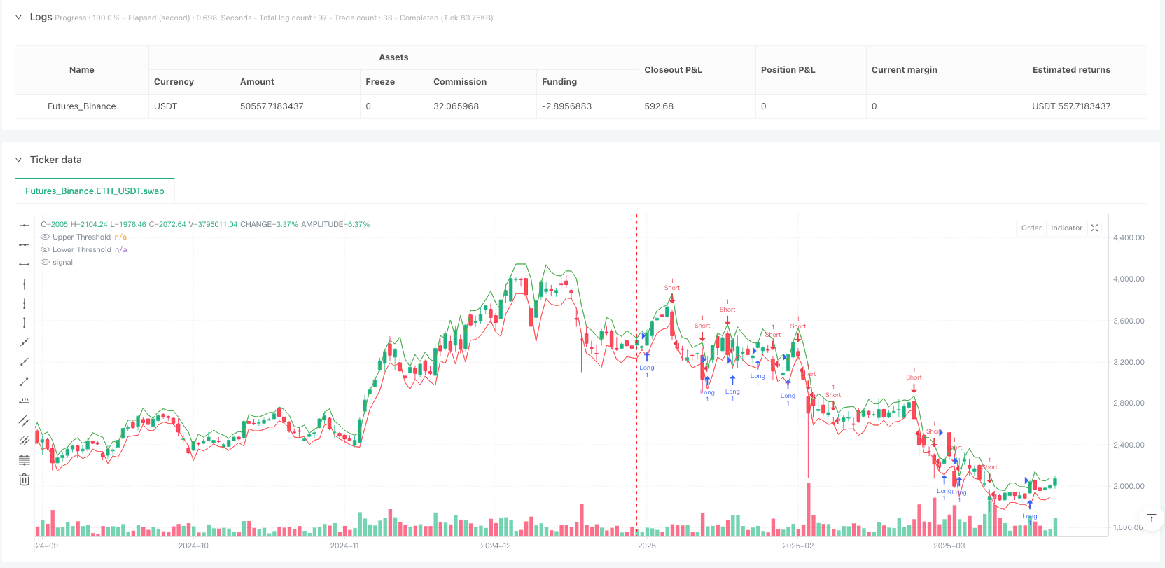
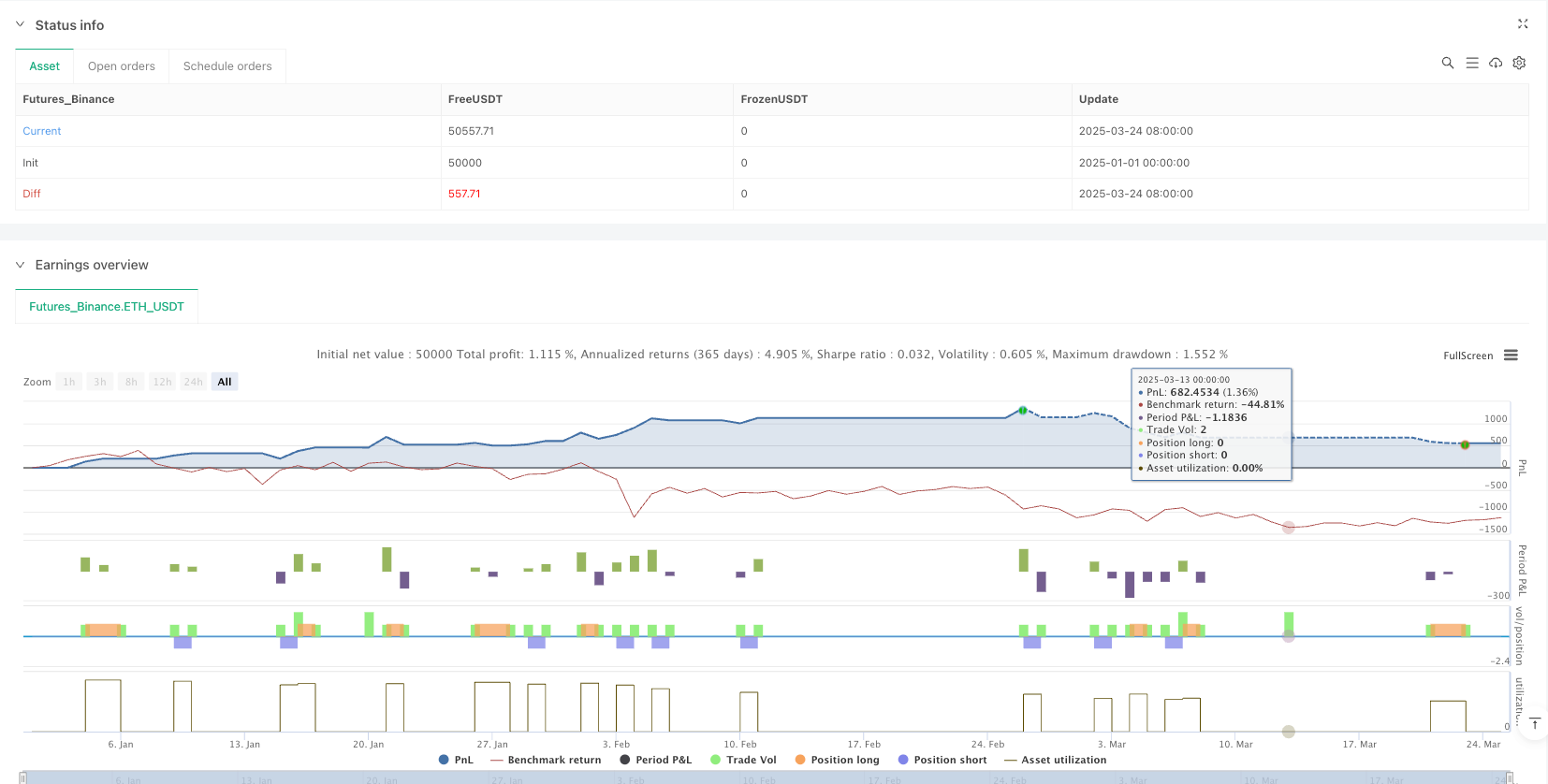
[trans]

概述

布莱克-斯科尔斯波动率调整动态突破策略是一种基于统计学和期权定价理论的量化交易方法。该策略巧妙地将布莱克-斯科尔斯模型的思想应用于市场价格突破分析中，通过计算历史波动率并动态调整预期价格区间，实现对突破信号的智能捕捉。策略的核心在于利用对数收益率的标准差来估算市场波动性，并将其转化为每个交易周期的预期价格变动幅度，从而建立动态的上下阈值，当价格突破这些阈值时触发相应的买入或卖出信号。同时，策略内置了止损和止盈机制，确保风险得到有效控制。

策略原理

该策略的运作原理基于以下步骤：

1. 波动率计算：首先计算历史收益的对数收益率（logReturn = math.log(close / close[1])），然后使用设定的回溯周期（默认20个周期）计算这些对数收益率的标准差，并将其年化（乘以交易周期的平方根，考虑每年252个交易日，每天390分钟）。

2. 预期移动计算：使用布莱克-斯科尔斯灵感的方法计算每个交易周期的预期价格变动（expectedMove = close[1] * volatility * math.sqrt(1 / periodsPerYear)）。这实际上是将年化波动率转换为单一周期的预期变动幅度。

3. 动态阈值设定：根据前一收盘价和计算出的预期移动幅度，设置上下两个阈值（upperThreshold = close[1] + expectedMove和lowerThreshold = close[1] - expectedMove）。

4. 交易信号生成：当当前收盘价突破上阈值时，触发做多信号；当突破下阈值时，触发做空信号。

5. 风险管理：策略在进入交易后自动设置基于百分比的止损（默认1%）和止盈（默认2%）。对于多头头寸，止损设在入场价格下方指定百分比处，止盈设在上方指定百分比处；空头头寸则相反。

优势分析

1. 动态适应性：相比使用固定价格或百分比的传统突破策略，该策略根据市场实际波动情况动态调整突破阈值，更能适应不同市场条件和波动环境。

2. 统计学基础：策略基于成熟的统计学原理和期权定价理论，使用对数收益率和标准差计算，理论基础扎实。

3. 自动风险管理：内置的止损和止盈机制确保每笔交易都有预设的风险控制措施，避免了因情绪因素导致的过度持仓或亏损扩大。

4. 参数灵活性：用户可以根据不同市场和个人风险偏好调整波动率回溯周期、止损和止盈百分比，使策略具有较高的适应性。

5. 计算效率：策略计算相对简单直接，无需复杂的指标组合，减少了过度拟合的风险，并提高了执行效率。

风险分析

1. 假突破风险：市场可能出现短暂突破阈值后迅速回撤的情况，导致错误信号和不必要的交易成本。可通过增加确认机制（如要求突破持续一定时间或结合成交量确认）来降低此风险。

2. 波动率估计误差：历史波动率不一定能准确预测未来波动，特别是在市场条件急剧变化时。可以考虑结合隐含波动率或使用GARCH等更复杂的波动率模型来提高预测准确性。

3. 参数敏感性：策略性能可能对波动率回溯周期、止损和止盈设置较为敏感。建议进行广泛的回测和参数优化，找到特定市场的最佳参数组合。

4. 趋势市场表现：在强趋势市场中，价格可能长期保持在一个方向移动，超出预期波动范围，导致错过重要趋势。可考虑结合趋势指标对策略进行补充。

5. 交易成本影响：频繁的突破信号可能导致过多交易，增加佣金和滑点成本。可以通过设置交易间隔或信号过滤器来减少交易频率。

优化方向

1. 波动率计算改进：可以探索使用指数加权移动平均（EWMA）或GARCH模型计算波动率，这些方法能更好地捕捉波动率的聚集效应和时变特性。改进代码可能如下：

// EWMA波动率计算
alpha = 0.94  // 衰减因子
ewmaVar = 0.0
ewmaVar := alpha * ewmaVar[1] + (1 - alpha) * logReturn * logReturn
ewmaVol = math.sqrt(ewmaVar) * math.sqrt(periodsPerYear)

2. 信号确认机制：添加成交量确认或价格动量确认，减少假突破风险：

volumeConfirmation = volume > ta.sma(volume, 20) * 1.5
momentumConfirmation = ta.rsi(close, 14) > 50 for longCondition or < 50 for shortCondition
longCondition := longCondition and volumeConfirmation and momentumConfirmation

3. 自适应止损机制：基于ATR（真实波动幅度）设置动态止损，更好地适应市场波动情况：

atrPeriod = 14
atrMultiplier = 2
atrValue = ta.atr(atrPeriod)
dynamicStopLoss = atrMultiplier * atrValue

4. 时间过滤：添加交易时间过滤，避开波动异常的市场开盘和收盘时段：

timeFilter = (hour >= 10 and hour < 15) or (hour == 15 and minute < 30)
longCondition := longCondition and timeFilter

5. 多周期确认：通过检查更高时间周期的方向来过滤与主要趋势相反的信号：

higherTimeframeClose = request.security(syminfo.tickerid, "60", close)
higherTimeframeTrend = ta.ema(higherTimeframeClose, 20) > ta.ema(higherTimeframeClose, 50)
longCondition := longCondition and higherTimeframeTrend
shortCondition := shortCondition and not higherTimeframeTrend

总结

布莱克-斯科尔斯波动率调整动态突破策略是一种融合了期权定价理论与传统突破交易方法的创新量化策略。它通过计算市场波动率并转化为预期价格变动范围，建立动态的交易阈值，有效地适应不同市场条件下的波动特性。策略的核心优势在于其统计学基础、动态适应性和内置风险管理机制，使其在多变的市场环境中具有潜在优势。

然而，该策略也面临着假突破、波动率估计误差和参数敏感性等挑战。通过引入波动率计算改进、信号确认机制、动态风险管理和多周期分析等优化措施，可以显著提升策略的稳定性和可靠性。特别是在高波动或快速变化的市场环境中，这些优化将帮助策略更好地识别有效信号并控制风险。

总体而言，布莱克-斯科尔斯波动率调整动态突破策略代表了一种将传统技术分析与现代金融理论相结合的有效尝试，为量化交易者提供了一个具有坚实理论基础、灵活性强且易于实施的交易框架。通过持续优化和适当调整，该策略有望在不同市场条件下实现稳健的表现。 ||

Overview

The Black-Scholes Volatility Adjusted Dynamic Breakout Strategy is a quantitative trading approach based on statistical principles and option pricing theory. This strategy cleverly applies concepts from the Black-Scholes model to market price breakout analysis, calculating historical volatility and dynamically adjusting expected price ranges to intelligently capture breakout signals. The core of the strategy lies in using the standard deviation of logarithmic returns to estimate market volatility and transform it into expected price movement for each trading period, thereby establishing dynamic upper and lower thresholds. When prices break through these thresholds, corresponding buy or sell signals are triggered. Additionally, the strategy incorporates built-in stop-loss and take-profit mechanisms to ensure effective risk control.

Strategy Principles

The operating principles of this strategy are based on the following steps:

1. Volatility Calculation: First, logarithmic returns are calculated (logReturn = math.log(close / close[1])), then the standard deviation of these log returns is computed using a specified lookback period (default 20 periods) and annualized (multiplied by the square root of trading periods, considering 252 trading days per year with 390 minutes per day).

2. Expected Move Calculation: Using a Black-Scholes inspired approach, the expected price movement for each trading period is calculated (expectedMove = close[1] * volatility * math.sqrt(1 / periodsPerYear)). This effectively converts annualized volatility into an expected movement magnitude for a single period.

3. Dynamic Threshold Setting: Based on the previous closing price and the calculated expected movement, upper and lower thresholds are established (upperThreshold = close[1] + expectedMove and lowerThreshold = close[1] - expectedMove).

4. Trading Signal Generation: When the current closing price breaks above the upper threshold, a long signal is triggered; when it breaks below the lower threshold, a short signal is triggered.

5. Risk Management: The strategy automatically sets percentage-based stop-loss (default 1%) and take-profit (default 2%) orders after entering a trade. For long positions, the stop-loss is set below the entry price by the specified percentage, and the take-profit above by the specified percentage; for short positions, the opposite applies.

Advantage Analysis

1. Dynamic Adaptability: Compared to traditional breakout strategies using fixed prices or percentages, this strategy dynamically adjusts breakout thresholds based on actual market volatility, better adapting to different market conditions and volatility environments.

2. Statistical Foundation: The strategy is based on established statistical principles and option pricing theory, using logarithmic returns and standard deviation calculations, providing a solid theoretical foundation.

3. Automated Risk Management: Built-in stop-loss and take-profit mechanisms ensure that each trade has preset risk control measures, avoiding excessive position holding or expanded losses due to emotional factors.

4. Parameter Flexibility: Users can adjust volatility lookback periods, stop-loss, and take-profit percentages according to different markets and personal risk preferences, giving the strategy high adaptability.

5. Computational Efficiency: The strategy calculations are relatively simple and direct, without requiring complex indicator combinations, reducing the risk of overfitting and improving execution efficiency.

Risk Analysis

1. False Breakout Risk: Markets may exhibit brief threshold breakouts followed by quick retracements, leading to false signals and unnecessary trading costs. This risk can be reduced by adding confirmation mechanisms (such as requiring sustained breakouts or volume confirmation).

2. Volatility Estimation Errors: Historical volatility may not accurately predict future volatility, especially during rapidly changing market conditions. Consider incorporating implied volatility or using more complex volatility models like GARCH to improve prediction accuracy.

3. Parameter Sensitivity: Strategy performance may be sensitive to volatility lookback periods, stop-loss, and take-profit settings. Extensive backtesting and parameter optimization are recommended to find the optimal parameter combination for specific markets.

4. Trend Market Performance: In strong trending markets, prices may continue moving in one direction beyond the expected volatility range, causing missed opportunities in important trends. Consider supplementing the strategy with trend indicators.

5. Trading Cost Impact: Frequent breakout signals may lead to excessive trading, increasing commission and slippage costs. Setting trade intervals or signal filters can reduce trading frequency.

Optimization Directions

1. Volatility Calculation Improvements: Explore using Exponentially Weighted Moving Average (EWMA) or GARCH models to calculate volatility, which better capture volatility clustering effects and time-varying characteristics. Improved code might look like:

// EWMA volatility calculation
alpha = 0.94  // decay factor
ewmaVar = 0.0
ewmaVar := alpha * ewmaVar[1] + (1 - alpha) * logReturn * logReturn
ewmaVol = math.sqrt(ewmaVar) * math.sqrt(periodsPerYear)

2. Signal Confirmation Mechanism: Add volume confirmation or price momentum confirmation to reduce false breakout risks:

volumeConfirmation = volume > ta.sma(volume, 20) * 1.5
momentumConfirmation = ta.rsi(close, 14) > 50 for longCondition or < 50 for shortCondition
longCondition := longCondition and volumeConfirmation and momentumConfirmation

3. Adaptive Stop-Loss Mechanism: Set dynamic stop-losses based on ATR (Average True Range) to better adapt to market volatility:

atrPeriod = 14
atrMultiplier = 2
atrValue = ta.atr(atrPeriod)
dynamicStopLoss = atrMultiplier * atrValue

4. Time Filtering: Add trading time filters to avoid abnormally volatile market opening and closing periods:

timeFilter = (hour >= 10 and hour < 15) or (hour == 15 and minute < 30)
longCondition := longCondition and timeFilter

5. Multi-timeframe Confirmation: Filter signals that contradict the main trend by checking higher timeframe directions:

higherTimeframeClose = request.security(syminfo.tickerid, "60", close)
higherTimeframeTrend = ta.ema(higherTimeframeClose, 20) > ta.ema(higherTimeframeClose, 50)
longCondition := longCondition and higherTimeframeTrend
shortCondition := shortCondition and not higherTimeframeTrend

Summary

The Black-Scholes Volatility Adjusted Dynamic Breakout Strategy is an innovative quantitative approach that merges option pricing theory with traditional breakout trading methods. By calculating market volatility and converting it into expected price movement ranges, it establishes dynamic trading thresholds that effectively adapt to volatility characteristics under different market conditions. The strategy's core strengths lie in its statistical foundation, dynamic adaptability, and built-in risk management mechanisms, giving it potential advantages in changing market environments.

However, the strategy also faces challenges such as false breakouts, volatility estimation errors, and parameter sensitivity. By introducing improvements in volatility calculation, signal confirmation mechanisms, dynamic risk management, and multi-timeframe analysis, the strategy's stability and reliability can be significantly enhanced. These optimizations will particularly help the strategy better identify effective signals and control risk in highly volatile or rapidly changing market environments.

Overall, the Black-Scholes Volatility Adjusted Dynamic Breakout Strategy represents an effective attempt to combine traditional technical analysis with modern financial theory, providing quantitative traders with a trading framework that has a solid theoretical foundation, strong flexibility, and ease of implementation. With continuous optimization and appropriate adjustments, this strategy has the potential to achieve robust performance under various market conditions. [/trans]

Source (PineScript)

/*backtest
start: 2025-01-01 00:00:00
end: 2025-03-25 00:00:00
period: 1d
basePeriod: 1d
exchanges: [{"eid":"Futures_Binance","currency":"ETH_USDT"}]
*/

//@version=5
strategy("black-scholes expected breakoout", overlay=true, initial_capital=100000, currency=currency.USD, calc_on_order_fills=true, calc_on_every_tick=true)

// User Inputs
chartRes     = input.int(title="Chart Timeframe in Minutes", defval=1, minval=1)
volLookback  = input.int(title="Volatility Lookback (bars)", defval=20, minval=1)
stopLossPerc = input.float(title="Stop Loss (%)", defval=1.0, minval=0.1, step=0.1)
takeProfitPerc = input.float(title="Take Profit (%)", defval=2.0, minval=0.1, step=0.1)

// Calculate periods per year based on chart timeframe (252 trading days * 390 minutes per day)
periodsPerYear = (252 * 390) / chartRes

// Calculate annualized volatility from log returns
logReturn  = math.log(close / close[1])
volatility = ta.stdev(logReturn, volLookback) * math.sqrt(periodsPerYear)

// Expected move for one bar: S * σ * √(1/periodsPerYear)
expectedMove   = close[1] * volatility * math.sqrt(1 / periodsPerYear)

// Define dynamic thresholds around the previous close
upperThreshold = close[1] + expectedMove
lowerThreshold = close[1] - expectedMove

// Plot thresholds for visual reference
plot(upperThreshold, color=color.green, title="Upper Threshold")
plot(lowerThreshold, color=color.red, title="Lower Threshold")

// Trading Signals: breakout of thresholds
longCondition  = close > upperThreshold
shortCondition = close < lowerThreshold

if (longCondition)
    strategy.entry("Long", strategy.long)
if (shortCondition)
    strategy.entry("Short", strategy.short)

// Fixed Risk Management Exit Orders
if (strategy.position_size > 0)
    strategy.exit("Exit Long", from_entry="Long", 
                  stop=close * (1 - stopLossPerc / 100), 
                  limit=close * (1 + takeProfitPerc / 100))
if (strategy.position_size < 0)
    strategy.exit("Exit Short", from_entry="Short", 
                  stop=close * (1 + stopLossPerc / 100), 
                  limit=close * (1 - takeProfitPerc / 100))

Detail

https://www.fmz.com/strategy/488267

Last Modified

2025-03-26 13:36:32