strategies/多时间框架自适应市场机制量化交易策略-Multi-Timeframe-Adaptive-Market-Regime-Quantitative-Trading-Strategy.md

Name

多时间框架自适应市场机制量化交易策略-Multi-Timeframe-Adaptive-Market-Regime-Quantitative-Trading-Strategy

Author

ianzeng123

Strategy Description

[trans]

概述

多时间框架自适应市场机制量化交易策略是一个基于多指标综合分析的高级量化交易系统，能够根据不同市场条件自动调整其交易策略。该策略利用人工智能自适应技术识别四种市场机制（趋势型、区间型、波动型和平静型），并根据当前市场状态动态调整交易参数。核心技术包括多时间框架分析、蜡烛图形态识别、动态风险管理以及自优化算法，为交易者提供了一个全面而灵活的交易工具。

策略原理

该策略的核心在于其多层次的市场分析框架，通过整合多个技术指标实现精准的市场状态检测和信号生成：

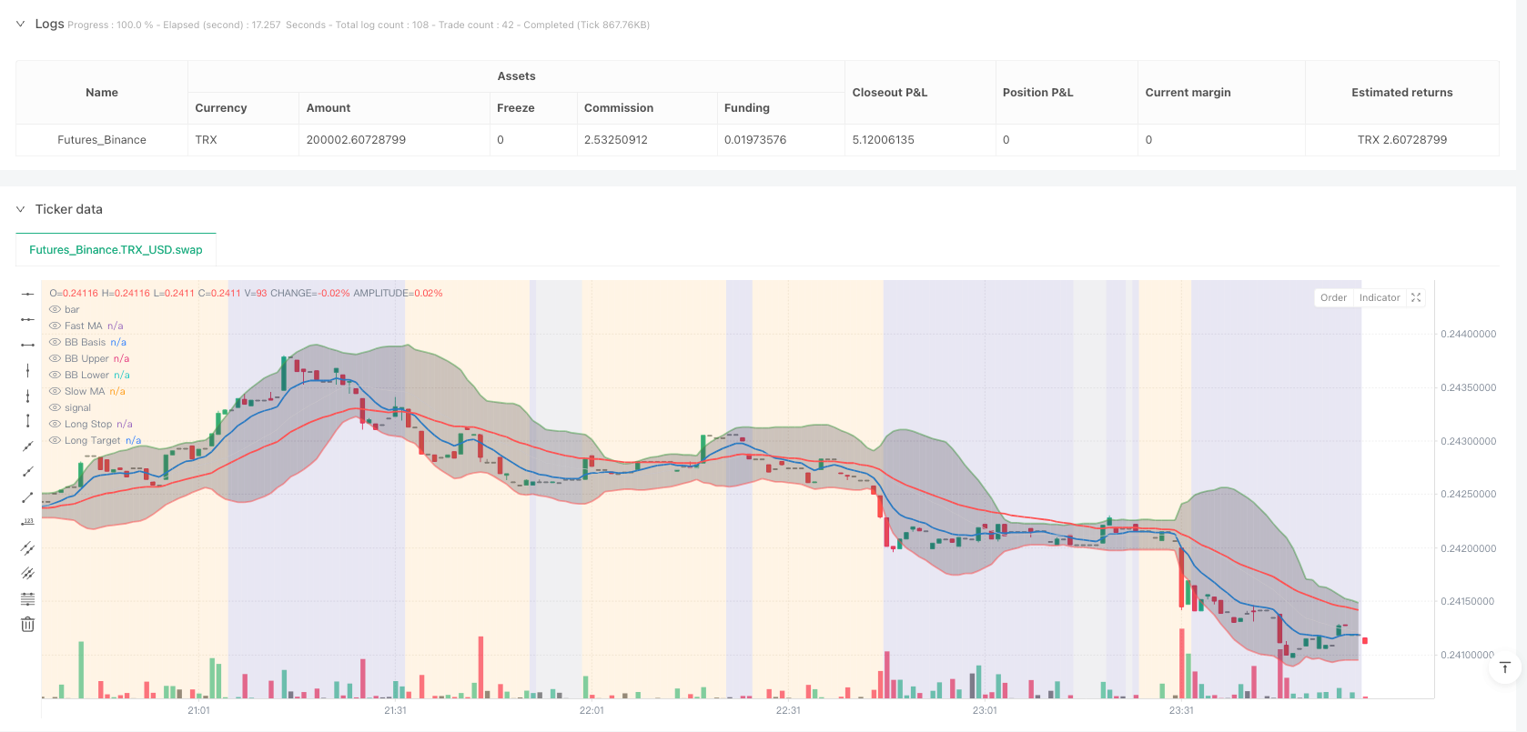
1. 移动平均线系统：使用快速（9周期）和慢速（34周期）指数移动平均线（EMA）确定趋势方向，结合ATR阈值增强判断准确性。

2. 多时间框架确认机制：通过更高时间周期的RSI和MACD指标提供更宏观的市场视角，过滤掉低时间周期的噪音信号。策略特别重视高时间框架的趋势确认，使用HTF_RSI和HTF_MACD的交叉点作为强力过滤器。

3. 市场机制识别算法：

   • 趋势型市场：ADX > 20且MA差距大于ATR的0.3倍，并得到高时间框架趋势确认
   • 区间型市场：ADX < 25且价格范围比率小于0.03，高时间框架中性
   • 波动型市场：布林带宽度大于平均宽度的1.5倍且ATR大于平均ATR的1.2倍
   • 平静型市场：布林带宽度小于平均宽度的0.8倍且ATR小于平均ATR的0.9倍

4. 蜡烛图形态识别与成交量确认：策略检测多种高概率蜡烛图形态，包括看涨吞没形态、锤子线、晨星形态、穿刺线、双底，以及其看跌对应形态。每个形态都需要成交量放大确认，增强信号可靠性。

5. 多因子评分系统：综合评估技术指标、形态识别和成交量情况，生成一个综合得分。买入信号要求牛市得分≥1.0，卖出信号要求熊市得分≥1.0。

6. 动态止损和追踪止损：使用ATR计算动态止损水平，确保风险管理适应市场波动性。止损距离根据ATR值自动调整，在波动性增加时扩大，在波动性降低时收缩。

7. 自优化性能追踪：系统记录不同市场机制下的交易表现，用于调整交易参数和评分阈值，实现策略的自适应优化。

策略优势

1. 全市场适应性：该策略最显著的优势是能够自动识别并适应四种不同的市场状态，避免了单一策略在变化的市场环境中的局限性。无论市场处于强烈趋势、横盘整理、高波动还是低波动状态，系统都能相应调整参数和信号阈值。

2. 多时间框架确认：通过整合更高时间周期的指标，策略显著提高了信号质量。这种"自上而下"的分析方法有效过滤了低质量信号，减少了假突破和噪音交易。

3. 高级形态识别：结合成交量确认的蜡烛图形态识别提供了高概率的入场信号。这些形态在支撑位和阻力位附近出现且伴随成交量放大时尤为有效。

4. 动态风险管理：基于ATR的止损和追踪止损机制确保了风险管理能够随市场波动性自动调整。这种方法在保护资本的同时，也允许盈利头寸继续运行，优化了风险回报比。

5. 自优化机制：策略能够记录在不同市场机制下的表现，为未来交易提供反馈和调整依据，实现不断自我完善。

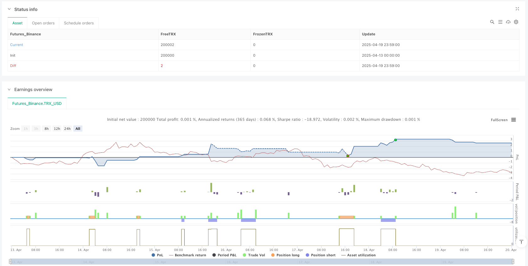
6. 可视化监控：通过颜色编码的背景和性能仪表板，交易者可以直观地了解当前市场状态、策略表现和关键指标，提高了操作透明度。

策略风险

1. 参数敏感性：该策略使用多个参数和阈值进行市场机制识别和信号生成。这些参数的设置需要谨慎调整，否则可能导致误判市场状态或生成错误信号。特别是ADX、ATR比率和布林带宽度等关键阈值需要根据不同交易品种的特性进行优化。

2. 计算复杂性：多层次的指标计算和逻辑判断增加了策略的复杂度，可能导致回测和实时执行速度变慢，尤其在低时间周期或高频交易环境下。

3. 市场转换延迟：尽管策略设计用于识别不同市场状态，但市场转换过程可能不是瞬时的，而是渐进的。在转换期间，策略可能面临误判和错误信号的风险。

4. 过度依赖技术指标：策略主要基于技术指标和价格形态，没有考虑基本面因素和市场情绪。在重大新闻或黑天鹅事件发生时，纯技术分析可能失效。

5. 回测偏差：由于策略的复杂性和自适应性，存在过度拟合历史数据的风险，实际表现可能不如回测结果。

6. 资本需求：动态风险管理机制可能在某些市场条件下需要较大的止损距离，这要求足够的交易资金以维持合理的风险比例。

优化方向

1. 机器学习增强：引入机器学习算法来优化市场机制识别和参数调整。可以使用历史数据训练模型，识别不同市场状态的潜在模式，提高分类准确性。实现方式可以包括使用随机森林或支持向量机进行市场状态分类，使用神经网络优化指标权重。

2. 情绪指标整合：引入市场情绪指标（如VIX、看跌/看涨期权比率、社交媒体情绪分析等）作为额外确认层。市场情绪数据可以作为领先指标，帮助预测市场转换点。

3. 基本面数据整合：开发一个框架来整合关键基本面数据，如经济日历事件、收益报告或重大新闻发布。这有助于在重要公告前调整风险敞口，避免意外波动带来的损失。

4. 时间过滤器：实施交易时段过滤器，避开流动性低或波动性异常的时段。这对于跨市场交易尤为重要，可以避免在亚洲、欧洲和美国市场交易时段交叉时段的异常行为。

5. 相关性分析模块：添加跨资产相关性分析功能，识别多市场模式和发散信号。例如，货币对之间的相关性、股指与VIX的关系等可以提供额外的交易确认。

6. 动态持仓规模优化：基于当前市场机制和历史绩效自动调整头寸规模。在表现良好的市场机制下可以增加风险敞口，在不确定或历史表现差的环境下降低风险。

7. 硬件优化：改进代码效率，减少计算复杂度，特别是在实时交易环境中。可以考虑重写部分逻辑，使用更高效的算法和数据结构。

总结

多时间框架自适应市场机制量化交易策略代表了量化交易系统的一次重要创新，将市场机制识别、多时间框架分析、形态识别和动态风险管理融为一体。其自适应能力和全面的技术指标整合使其能够在各种市场环境中保持竞争力，而不仅仅局限于单一市场状态。

该策略的真正价值在于其整体框架而非单个组件。通过市场机制识别、多时间框架确认、形态识别和动态风险管理的协同作用，策略能够生成高质量信号并有效管理风险。这种多层次方法减少了错误信号并提高了整体稳健性。

然而，该策略也面临参数敏感性、计算复杂性和潜在过度拟合等挑战。交易者在应用此策略时应注意这些风险，进行充分的参数优化和前向测试。

未来的优化方向包括机器学习增强、情绪指标整合和动态持仓规模调整等。这些改进将进一步提高策略的适应性和稳健性，使其成为一个更全面的交易系统。总体而言，该策略提供了一个强大的框架，可以根据交易者的风险偏好和市场观点进行定制和扩展。 ||

Overview

The Multi-Timeframe Adaptive Market Regime Quantitative Trading Strategy is an advanced quantitative trading system that leverages multi-indicator comprehensive analysis to automatically adjust its trading approach based on different market conditions. This strategy utilizes AI adaptive technology to identify four market regimes (trending, ranging, volatile, and quiet) and dynamically adjusts trading parameters according to the current market state. Core technologies include multi-timeframe analysis, candlestick pattern recognition, dynamic risk management, and self-optimization algorithms, providing traders with a comprehensive and flexible trading tool.

Strategy Principles

The core of this strategy lies in its multi-layered market analysis framework, which integrates multiple technical indicators to achieve precise market state detection and signal generation:

1. Moving Average System: Uses fast (9-period) and slow (34-period) exponential moving averages (EMAs) to determine trend direction, enhanced with ATR thresholds for improved accuracy.

2. Multi-Timeframe Confirmation Mechanism: Provides a more macro market perspective through higher timeframe RSI and MACD indicators, filtering out noise signals from lower timeframes. The strategy places special emphasis on higher timeframe trend confirmation, using HTF_RSI and HTF_MACD crossover points as powerful filters.

3. Market Regime Identification Algorithm:

   • Trending Market: ADX > 20 and MA difference greater than 0.3 times ATR, with higher timeframe trend confirmation
   • Ranging Market: ADX < 25 and price range ratio less than 0.03, neutral in higher timeframe
   • Volatile Market: Bollinger Band width greater than 1.5 times average width and ATR greater than 1.2 times average ATR
   • Quiet Market: Bollinger Band width less than 0.8 times average width and ATR less than 0.9 times average ATR

4. Candlestick Pattern Recognition with Volume Confirmation: The strategy detects multiple high-probability candlestick patterns, including bullish engulfing, hammer, morning star, piercing line, double bottom, and their bearish counterparts. Each pattern requires volume expansion confirmation to enhance signal reliability.

5. Multi-Factor Scoring System: Comprehensively evaluates technical indicators, pattern recognition, and volume conditions to generate a composite score. Buy signals require a bullish score ≥ 1.0, while sell signals require a bearish score ≥ 1.0.

6. Dynamic Stop-Loss and Trailing Stops: Uses ATR to calculate dynamic stop-loss levels, ensuring risk management adapts to market volatility. Stop-loss distances automatically adjust based on ATR values, expanding during increased volatility and contracting during decreased volatility.

7. Self-Optimizing Performance Tracking: The system records trading performance across different market regimes, used to adjust trading parameters and scoring thresholds, achieving strategy self-adaptation and optimization.

Strategy Advantages

1. Full Market Adaptability: The most significant advantage of this strategy is its ability to automatically identify and adapt to four different market states, avoiding the limitations of single strategies in changing market environments. Whether the market is in a strong trend, consolidation, high volatility, or low volatility, the system can adjust parameters and signal thresholds accordingly.

2. Multi-Timeframe Confirmation: By integrating indicators from higher timeframes, the strategy significantly improves signal quality. This "top-down" analysis method effectively filters out low-quality signals, reducing false breakouts and noise trades.

3. Advanced Pattern Recognition: Candlestick pattern recognition combined with volume confirmation provides high-probability entry signals. These patterns are particularly effective when appearing near support and resistance levels with accompanying volume expansion.

4. Dynamic Risk Management: ATR-based stop-loss and trailing stop mechanisms ensure that risk management can automatically adjust with market volatility. This approach protects capital while allowing profitable positions to continue running, optimizing the risk-reward ratio.

5. Self-Optimization Mechanism: The strategy can record performance across different market regimes, providing feedback and adjustment basis for future trades, achieving continuous self-improvement.

6. Visual Monitoring: Through color-coded backgrounds and performance dashboards, traders can intuitively understand the current market state, strategy performance, and key indicators, improving operational transparency.

Strategy Risks

1. Parameter Sensitivity: The strategy uses multiple parameters and thresholds for market regime identification and signal generation. These parameters need to be carefully adjusted, otherwise they may lead to misjudgment of market states or generate incorrect signals. Key thresholds such as ADX, ATR ratio, and Bollinger Band width need to be optimized according to the characteristics of different trading instruments.

2. Computational Complexity: Multi-layered indicator calculations and logical judgments increase the strategy's complexity, potentially slowing down backtesting and real-time execution, especially in lower timeframes or high-frequency trading environments.

3. Market Transition Delay: Although the strategy is designed to identify different market states, market transitions may not be instantaneous but gradual. During transitions, the strategy may face risks of misjudgment and false signals.

4. Over-reliance on Technical Indicators: The strategy is primarily based on technical indicators and price patterns, without considering fundamental factors and market sentiment. Pure technical analysis may fail during major news or black swan events.

5. Backtesting Bias: Due to the strategy's complexity and adaptability, there is a risk of overfitting historical data, and actual performance may not match backtesting results.

6. Capital Requirements: The dynamic risk management mechanism may require larger stop-loss distances under certain market conditions, requiring sufficient trading capital to maintain reasonable risk proportions.

Optimization Directions

1. Machine Learning Enhancement: Introduce machine learning algorithms to optimize market regime identification and parameter adjustment. Historical data can be used to train models to identify potential patterns in different market states and improve classification accuracy. Implementation methods can include using random forests or support vector machines for market state classification, and neural networks for optimizing indicator weights.

2. Sentiment Indicator Integration: Introduce market sentiment indicators (such as VIX, put/call ratios, social media sentiment analysis, etc.) as additional confirmation layers. Market sentiment data can serve as leading indicators, helping predict market transition points.

3. Fundamental Data Integration: Develop a framework to integrate key fundamental data, such as economic calendar events, earnings reports, or major news releases. This helps adjust risk exposure before important announcements, avoiding losses from unexpected volatility.

4. Time Filters: Implement trading session filters to avoid periods of low liquidity or abnormal volatility. This is particularly important for cross-market trading, avoiding abnormal behavior during the crossover periods of Asian, European, and American market trading sessions.

5. Correlation Analysis Module: Add cross-asset correlation analysis functionality to identify multi-market patterns and divergence signals. For example, correlations between currency pairs, relationships between stock indices and VIX, etc., can provide additional trade confirmations.

6. Dynamic Position Sizing Optimization: Automatically adjust position size based on current market regime and historical performance. Risk exposure can be increased in well-performing market regimes and reduced in uncertain or historically poor-performing environments.

7. Hardware Optimization: Improve code efficiency and reduce computational complexity, especially in real-time trading environments. Consider rewriting portions of logic using more efficient algorithms and data structures.

Summary

The Multi-Timeframe Adaptive Market Regime Quantitative Trading Strategy represents a significant innovation in quantitative trading systems, integrating market regime identification, multi-timeframe analysis, pattern recognition, and dynamic risk management. Its adaptive capability and comprehensive technical indicator integration allow it to remain competitive across various market environments, not just limited to a single market state.

The true value of this strategy lies in its overall framework rather than individual components. Through the synergy of market regime identification, multi-timeframe confirmation, pattern recognition, and dynamic risk management, the strategy can generate high-quality signals and effectively manage risk. This multi-layered approach reduces false signals and enhances overall robustness.

However, the strategy also faces challenges such as parameter sensitivity, computational complexity, and potential overfitting. Traders should be aware of these risks when applying this strategy, conducting thorough parameter optimization and forward testing.

Future optimization directions include machine learning enhancement, sentiment indicator integration, and dynamic position sizing adjustment. These improvements will further enhance the strategy's adaptability and robustness, making it a more comprehensive trading system. Overall, this strategy provides a powerful framework that can be customized and expanded according to traders' risk preferences and market views.[/trans]

Source (PineScript)

/*backtest
start: 2025-04-13 00:00:00
end: 2025-04-20 00:00:00
period: 1m
basePeriod: 1m
exchanges: [{"eid":"Futures_Binance","currency":"TRX_USD"}]
*/

//@version=6
strategy("Dskyz (DAFE) AI Adaptive Regime - Pro", overlay=true, default_qty_type=strategy.fixed, default_qty_value=1, calc_on_order_fills=true, calc_on_every_tick=true)

// This script uses higher timeframe values for RSI/MACD, integrated into regime detection and scoring.
// Logic uses closed HTF bars to avoid repainting.

// D=====================================================Z
// 1. ATR SETTINGS==Z
// D=====================================================Z
group_atr = "⚡ ATR Settings"
atr_period     = input.int(14, "ATR Period", minval=1, group=group_atr)
atr_multiplier = input.float(1.5, "ATR Multiplier", minval=0.1, step=0.1, group=group_atr)
atr_val        = ta.atr(atr_period)
atr_avg        = ta.sma(atr_val, 50)

// D=====================================================Z
// 2. MOVING AVERAGE (MA) SETTINGS==Z
// D=====================================================Z
group_ma = "? Moving Averages"
fast_ma_length        = input.int(9, "Fast MA Length", minval=1, group=group_ma)
slow_ma_length        = input.int(34, "Slow MA Length", minval=1, group=group_ma)
ma_fast               = ta.ema(close, fast_ma_length)
ma_slow               = ta.ema(close, slow_ma_length)
ma_strength_threshold = input.float(0.5, "MA Strength Threshold", minval=0.0, step=0.1, group=group_ma)
trend_dir = ma_fast > ma_slow + (atr_val * ma_strength_threshold) ? 1 : ma_fast < ma_slow - (atr_val * ma_strength_threshold) ? -1 : 0

// D=====================================================Z
// 3. MULTI-TIMEFRAME (HTF) SETTINGS==Z
// D=====================================================Z
group_MTA = "⏱️ Multi-Timeframe Inputs"
htf = input.timeframe("D", "HTF for RSI & MACD", group=group_MTA)
htf_rsi_raw = request.security(syminfo.tickerid, htf, ta.rsi(close, 14))
htf_rsi = htf_rsi_raw[1]
[htf_macd_line_raw, htf_macd_signal_raw, htf_macd_hist_raw] = request.security(syminfo.tickerid, htf, ta.macd(close, 12, 26, 9))
htf_macd_line = htf_macd_line_raw[1]
htf_macd_signal = htf_macd_signal_raw[1]
htf_macd_hist = htf_macd_hist_raw[1]
// new: HTF trend direction for regime detection
htf_trend_bull = htf_macd_line > htf_macd_signal and htf_rsi > 50
htf_trend_bear = htf_macd_line < htf_macd_signal and htf_rsi < 50

// D=====================================================Z
// 4. TRADE SETTINGS==Z
// D=====================================================Z
group_trade = "⚙️ Trade Settings"
risk_per_trade      = input.int(500, "Risk per Trade ($)", minval=50, group=group_trade)
max_contracts       = input.int(5, "Max Contracts", minval=1, group=group_trade)
max_daily_drawdown  = input.float(0.05, "Max Daily Drawdown (%)", minval=0.01, group=group_trade)
tick_value          = input.float(12.5, "Tick Value ($)", minval=0.01, group=group_trade)
ticks_per_point     = input.int(4, "Ticks per Point", minval=1, group=group_trade)
default_stop_points = input.float(8.0, "Default Stop (Points)", minval=0.25, group=group_trade)

// D=====================================================Z
// 5. ADVANCED INDICATOR CALCULATIONS==Z
// D=====================================================Z

// --- ADX Calculation ---Z
adx_len   = 14
up        = ta.change(high)
down      = -ta.change(low)
plus_dm   = na(up) ? na : (up > down and up > 0 ? up : 0)
minus_dm  = na(down) ? na : (down > up and down > 0 ? down : 0)
trur      = ta.rma(ta.tr, adx_len)
plus_di   = 100 * ta.rma(plus_dm, adx_len) / trur
minus_di  = 100 * ta.rma(minus_dm, adx_len) / trur
adx_val   = 100 * ta.rma(math.abs(plus_di - minus_di) / (plus_di + minus_di), adx_len)

// --- Bollinger Bands Calculation ---Z
bb_basis     = ta.sma(close, 20)
bb_dev       = 2 * ta.stdev(close, 20)
bb_upper     = bb_basis + bb_dev
bb_lower     = bb_basis - bb_dev
bb_width     = (bb_upper - bb_lower) / bb_basis
bb_width_avg = ta.sma(bb_width, 50)

// --- Price Action Range ---Z
price_range = ta.highest(high, 20) - ta.lowest(low, 20)
range_ratio = price_range / close

// D=====================================================Z
// 6. REGIME ASSIGNMENT & PATTERN RECOGNITION==Z
// D=====================================================Z

// Regime assignment with HTF influence and looser thresholds
is_trending = adx_val > 20 and math.abs(ma_fast - ma_slow) > atr_val * 0.3 and htf_trend_bull or htf_trend_bear // loosened ADX and MA thresholds, added HTF
is_range    = adx_val < 25 and range_ratio < 0.03 and not htf_trend_bull and not htf_trend_bear // loosened ADX and range, HTF neutral
is_volatile = bb_width > bb_width_avg * 1.5 and atr_val > atr_avg * 1.2 and (htf_rsi > 70 or htf_rsi < 30) // loosened BB/ATR, added HTF overbought/oversold
is_quiet    = bb_width < bb_width_avg * 0.8 and atr_val < atr_avg * 0.9 // loosened BB/ATR
regime      = is_trending ? 1 : is_range ? 2 : is_volatile ? 3 : is_quiet ? 4 : 5
regime_name = regime == 1 ? "Trending" : regime == 2 ? "Range" : regime == 3 ? "Volatile" : regime == 4 ? "Quiet" : "Other"

// Pattern Recognition & Volume Confirmation-Z
vol_avg       = ta.sma(volume, 20)
vol_spike     = volume > vol_avg * 1.5
recent_low    = ta.lowest(low, 20)
recent_high   = ta.highest(high, 20)
is_near_support    = low <= recent_low * 1.01
is_near_resistance = high >= recent_high * 0.99

bullish_engulfing = close[1] < open[1] and close > open and close > open[1] and open < close[1] and is_near_support and vol_spike
hammer            = high - low > 3 * math.abs(open - close) and (close - low) / (0.001 + high - low) > 0.6 and is_near_support and vol_spike
morning_star      = close[2] < open[2] and math.abs(close[1] - open[1]) < 0.2 * (high[1] - low[1]) and close > open and close > (open[2] + close[2]) / 2 and is_near_support and vol_spike
piercing          = close[1] < open[1] and close > open and close > (open[1] + close[1]) / 2 and open < close[1] and is_near_support and vol_spike
double_bottom     = low < low[1] and low[1] > low[2] and low[2] < low[3] and close > open and is_near_support and vol_spike

bearish_engulfing = close[1] > open[1] and close < open and close < open[1] and open > close[1] and is_near_resistance and vol_spike
shooting_star     = high - low > 3 * math.abs(open - close) and (high - close) / (0.001 + high - low) > 0.6 and is_near_resistance and vol_spike
evening_star      = close[2] > open[2] and math.abs(close[1] - open[1]) < 0.2 * (high[1] - low[1]) and close < open and close < (open[2] + close[2]) / 2 and is_near_resistance and vol_spike
dark_cloud        = close[1] > open[1] and close < open and close < (open[1] + close[1]) / 2 and open > close[1] and is_near_resistance and vol_spike
double_top        = high > high[1] and high[1] < high[2] and high[2] > high[3] and close < open and is_near_resistance and vol_spike

bull_signal = (bullish_engulfing ? 0.5 : 0.0) +
              (hammer ? (regime == 2 ? 0.4 : 0.2) : 0.0) +
              (morning_star ? 0.2 : 0.0) +
              (piercing ? 0.2 : 0.0) +
              (double_bottom ? (regime == 3 ? 0.3 : 0.15) : 0.0)

bear_signal = (bearish_engulfing ? 0.5 : 0.0) +
              (shooting_star ? (regime == 2 ? 0.4 : 0.2) : 0.0) +
              (evening_star ? 0.2 : 0.0) +
              (dark_cloud ? 0.2 : 0.0) +
              (double_top ? (regime == 3 ? 0.3 : 0.15) : 0.0)

// Multi-Factor Confirmation with HTF-Z
rsi_val   = ta.rsi(close, 14)
[macd_line, macd_signal, macd_hist] = ta.macd(close, 12, 26, 9)
trend_bull = ma_fast > ma_slow
trend_bear = ma_fast < ma_slow
rsi_bull   = rsi_val < 30
rsi_bear   = rsi_val > 70
macd_bull  = macd_line > macd_signal
macd_bear  = macd_line < macd_signal
vol_expansion = atr_val > atr_avg * 1.2
// new: HTF confirmation for scoring
htf_bull_confirm = htf_trend_bull and htf_rsi < 70
htf_bear_confirm = htf_trend_bear and htf_rsi > 30

bull_score = bull_signal + (trend_bull ? 0.2 : 0) + (rsi_bull ? 0.15 : 0) + (macd_bull ? 0.15 : 0) + (vol_expansion ? 0.1 : 0) + (htf_bull_confirm ? 0.2 : 0)
bear_score = bear_signal + (trend_bear ? 0.2 : 0) + (rsi_bear ? 0.15 : 0) + (macd_bear ? 0.15 : 0) + (vol_expansion ? 0.1 : 0) + (htf_bear_confirm ? 0.2 : 0)

// D=====================================================Z
// 7. PERFORMANCE TRACKING & ADAPTIVE THRESHOLDS==Z
// D=====================================================Z
var float[] regime_pnl_long  = array.new_float(5, 0)
var float[] regime_pnl_short = array.new_float(5, 0)
var int[] regime_win_long    = array.new_int(5, 0)
var int[] regime_loss_long   = array.new_int(5, 0)
var int[] regime_win_short   = array.new_int(5, 0)
var int[] regime_loss_short  = array.new_int(5, 0)
var int entry_regime = na

if barstate.isconfirmed and strategy.closedtrades > 0 and not na(entry_regime)
    last_trade_profit = strategy.closedtrades.profit(strategy.closedtrades - 1)
    last_trade_entry_id = strategy.closedtrades.entry_id(strategy.closedtrades - 1)
    idx = entry_regime - 1
    if last_trade_entry_id == "Long"
        array.set(regime_pnl_long, idx, array.get(regime_pnl_long, idx) + last_trade_profit)
        if last_trade_profit > 0
            array.set(regime_win_long, idx, array.get(regime_win_long, idx) + 1)
        else
            array.set(regime_loss_long, idx, array.get(regime_loss_long, idx) + 1)
    else if last_trade_entry_id == "Short"
        array.set(regime_pnl_short, idx, array.get(regime_pnl_short, idx) + last_trade_profit)
        if last_trade_profit > 0
            array.set(regime_win_short, idx, array.get(regime_win_short, idx) + 1)
        else
            array.set(regime_loss_short, idx, array.get(regime_loss_short, idx) + 1)
    entry_regime := na

// D=====================================================Z
// 8. DRAWDOWN & CIRCUIT BREAKER==Z
// D=====================================================Z
var float max_equity = strategy.equity
if strategy.equity > max_equity
    max_equity := strategy.equity
daily_drawdown = (max_equity - strategy.equity) / max_equity
pause_trading  = daily_drawdown > max_daily_drawdown

// D=====================================================Z
// 9. ENTRY & EXIT LOGIC WITH DYNAMIC STOPS & TRAILING STOPS=Z
// D=====================================================Z
swing_low  = ta.lowest(low, 5)
swing_high = ta.highest(high, 5)
long_condition  = bull_score >= 1.0 and not pause_trading
short_condition = bear_score >= 1.0 and not pause_trading

var float trail_stop_long  = na
var float trail_stop_short = na
var float long_stop_price  = na
var float long_limit_price = na
var float short_stop_price = na
var float short_limit_price = na

if long_condition and strategy.position_size <= 0
    intended_stop = swing_low - atr_multiplier * atr_val
    stop_distance_points = close - intended_stop
    risk_per_contract = stop_distance_points * syminfo.pointvalue
    contracts = math.floor(risk_per_trade / risk_per_contract)
    contracts := contracts > 0 ? contracts : 1
    contracts := math.min(contracts, max_contracts)
    long_limit = close + stop_distance_points * 2
    strategy.entry("Long", strategy.long, qty = contracts)
    strategy.exit("Exit", from_entry = "Long", stop = intended_stop, limit = long_limit)
    long_stop_price  := intended_stop
    long_limit_price := long_limit
    trail_stop_long  := intended_stop
    entry_regime     := regime

if short_condition and strategy.position_size >= 0
    intended_stop = swing_high + atr_multiplier * atr_val
    stop_distance_points = intended_stop - close
    risk_per_contract = stop_distance_points * syminfo.pointvalue
    contracts = math.floor(risk_per_trade / risk_per_contract)
    contracts := contracts > 0 ? contracts : 1
    contracts := math.min(contracts, max_contracts)
    short_limit = close - stop_distance_points * 2
    strategy.entry("Short", strategy.short, qty = contracts)
    strategy.exit("Exit", from_entry = "Short", stop = intended_stop, limit = short_limit)
    short_stop_price  := intended_stop
    short_limit_price := short_limit
    trail_stop_short  := intended_stop
    entry_regime      := regime

if strategy.position_size > 0
    if close > long_limit_price * 0.5
        trail_stop_long := math.max(trail_stop_long, close - atr_val * atr_multiplier)
    strategy.exit("Long Trailing Stop", from_entry = "Long", stop = trail_stop_long)

if strategy.position_size < 0
    if close < short_limit_price * 0.5
        trail_stop_short := math.min(trail_stop_short, close + atr_val * atr_multiplier)
    strategy.exit("Short Trailing Stop", from_entry = "Short", stop = trail_stop_short)

if strategy.position_size == 0
    long_stop_price  := na
    long_limit_price := na
    short_stop_price := na
    short_limit_price := na

// D=====================================================Z
// 10. VISUALIZATION==Z
// D=====================================================Z
bgcolor(regime == 1 ? color.new(color.green, 85) : 
       regime == 2 ? color.new(color.orange, 85) : 
       regime == 3 ? color.new(color.red, 85) : 
       regime == 4 ? color.new(color.gray, 85) : 
       color.new(color.navy, 85))

plotshape(long_condition, style=shape.triangleup, location=location.belowbar, color=color.green, size=size.small, title="Long Signal")
plotshape(short_condition, style=shape.triangledown, location=location.abovebar, color=color.red, size=size.small, title="Short Signal")
plot(ma_fast, "Fast MA", color=color.new(color.blue, 0), linewidth=2)
plot(ma_slow, "Slow MA", color=color.new(color.red, 0), linewidth=2)
plot(strategy.position_size > 0 ? long_stop_price  : na, "Long Stop", color=color.new(color.red, 0), style=plot.style_linebr)
plot(strategy.position_size > 0 ? long_limit_price : na, "Long Target", color=color.new(color.green, 0), style=plot.style_linebr)
plot(strategy.position_size < 0 ? short_stop_price  : na, "Short Stop", color=color.new(color.red, 0), style=plot.style_linebr)
plot(strategy.position_size < 0 ? short_limit_price : na, "Short Target", color=color.new(color.green, 0), style=plot.style_linebr)

// D=====================================================Z
// 11. DASHBOARD: METRICS TABLE (Bottom-Left)=Z
// D=====================================================Z
var table dashboard = table.new(position.bottom_left, 2, 13, bgcolor=color.new(#000000, 29), border_color=color.rgb(80,80,80), border_width=1)
if barstate.islast
    table.cell(dashboard, 0, 0, "⚡(DAFE) AI Adaptive Regime™", text_color=color.rgb(96,8,118), text_size=size.small)
    modeStr = pause_trading ? "Paused" : "Active"
    table.cell(dashboard, 0, 1, "Mode:", text_color=color.white, text_size=size.small)
    table.cell(dashboard, 1, 1, modeStr, text_color=color.white, text_size=size.small)
    trendText = trend_dir == 1 ? "Bullish" : trend_dir == -1 ? "Bearish" : "Neutral"
    table.cell(dashboard, 0, 2, "Trend:", text_color=color.white, text_size=size.small)
    table.cell(dashboard, 1, 2, trendText, text_color=trend_dir == 1 ? color.green : trend_dir == -1 ? color.red : color.gray, text_size=size.small)
    table.cell(dashboard, 0, 3, "ATR:", text_color=color.white, text_size=size.small)
    table.cell(dashboard, 1, 3, str.tostring(atr_val, "#.##"), text_color=color.white, text_size=size.small)
    table.cell(dashboard, 0, 4, "ATR Avg:", text_color=color.white, text_size=size.small)
    table.cell(dashboard, 1, 4, str.tostring(atr_avg, "#.##"), text_color=color.white, text_size=size.small)
    table.cell(dashboard, 0, 5, "Volume Spike:", text_color=color.white, text_size=size.small)
    table.cell(dashboard, 1, 5, vol_spike ? "YES" : "NO", text_color=vol_spike ? color.green : color.red, text_size=size.small)
    table.cell(dashboard, 0, 6, "RSI:", text_color=color.white, text_size=size.small)
    table.cell(dashboard, 1, 6, str.tostring(rsi_val, "#.##"), text_color=color.white, text_size=size.small)
    rsiCondText = rsi_val < 30 ? "Oversold" : rsi_val > 70 ? "Overbought" : "Neutral"
    table.cell(dashboard, 0, 7, "RSI Cond:", text_color=color.white, text_size=size.small)
    table.cell(dashboard, 1, 7, rsiCondText, text_color=color.white, text_size=size.small)
    table.cell(dashboard, 0, 8, "HTF RSI:", text_color=color.white, text_size=size.small)
    table.cell(dashboard, 1, 8, str.tostring(htf_rsi, "#.##"), text_color=color.white, text_size=size.small)
    htfTrendText = htf_trend_bull ? "Bullish" : htf_trend_bear ? "Bearish" : "Neutral"
    table.cell(dashboard, 0, 9, "HTF Trend:", text_color=color.white, text_size=size.small)
    table.cell(dashboard, 1, 9, htfTrendText, text_color=htf_trend_bull ? color.green : htf_trend_bear ? color.red : color.gray, text_size=size.small)
    lastSignal = long_condition ? "Buy" : short_condition ? "Sell" : "None"
    table.cell(dashboard, 0, 10, "Last Signal:", text_color=color.white, text_size=size.small)
    table.cell(dashboard, 1, 10, lastSignal, text_color=long_condition ? color.green : short_condition ? color.red : color.white, text_size=size.small)
    table.cell(dashboard, 0, 11, "Regime:", text_color=color.white, text_size=size.small)
    table.cell(dashboard, 1, 11, regime_name, text_color=color.white, text_size=size.small)
    table.cell(dashboard, 0, 12, "Bull Score:", text_color=color.white, text_size=size.small)
    table.cell(dashboard, 1, 12, str.tostring(bull_score, "#.##"), text_color=color.white, text_size=size.small)

// D=====================================================Z
// REGIME CONDITIONS
// D=====================================================Z
var table debug_table = table.new(position.top_right, 2, 5, bgcolor=color.new(#000000, 50), border_color=color.rgb(80,80,80), border_width=1)
if barstate.islast
    table.cell(debug_table, 0, 0, "Regime Conditions", text_color=color.rgb(96,8,118), text_size=size.small)
    table.cell(debug_table, 0, 1, "ADX:", text_color=color.white, text_size=size.small)
    table.cell(debug_table, 1, 1, str.tostring(adx_val, "#.##"), text_color=color.white, text_size=size.small)
    table.cell(debug_table, 0, 2, "BB Width Ratio:", text_color=color.white, text_size=size.small)
    table.cell(debug_table, 1, 2, str.tostring(bb_width / bb_width_avg, "#.##"), text_color=color.white, text_size=size.small)
    table.cell(debug_table, 0, 3, "ATR Ratio:", text_color=color.white, text_size=size.small)
    table.cell(debug_table, 1, 3, str.tostring(atr_val / atr_avg, "#.##"), text_color=color.white, text_size=size.small)
    table.cell(debug_table, 0, 4, "Range Ratio:", text_color=color.white, text_size=size.small)
    table.cell(debug_table, 1, 4, str.tostring(range_ratio, "#.##"), text_color=color.white, text_size=size.small)

// --- Bollinger Bands Visuals ---Z
p_bb_basis = plot(bb_basis, title="BB Basis", color=color.new(#ffffff, 50), linewidth=1)
p_bb_upper = plot(bb_upper, title="BB Upper", color=color.new(#4caf4f, 45), linewidth=2)
p_bb_lower = plot(bb_lower, title="BB Lower", color=color.new(#ff5252, 45), linewidth=2)
fill(p_bb_upper, p_bb_lower, color=color.new(#423645, 65))

//D=================================================================Z
// DASHBOARD: WATERMARK LOGO (Bottom-Right)
//D=================================================================Z
var table watermarkTable = table.new(position.bottom_right, 1, 1, bgcolor=color.rgb(0,0,0,80), border_color=color.rgb(0,50,137), border_width=1)
if barstate.islast
    table.cell(watermarkTable, 0, 0, "⚡ Dskyz (DAFE) AI Adaptive Regime - Pro", text_color=color.rgb(96,8,118), text_size=size.normal)

// --- ALERTS ---Z
alertcondition(long_condition, title="Long Signal Alert", message="Enhanced Strategy Long Signal")
alertcondition(short_condition, title="Short Signal Alert", message="Enhanced Strategy Short Signal")

Detail

https://www.fmz.com/strategy/491512

Last Modified

2025-04-21 16:20:34