strategies/多周期波动跟踪量化策略-Multi-Timeframe-Volatility-Tracking-Quantitative-Strategy.md

Name

多周期波动跟踪量化策略-Multi-Timeframe-Volatility-Tracking-Quantitative-Strategy

Author

ianzeng123

Strategy Description

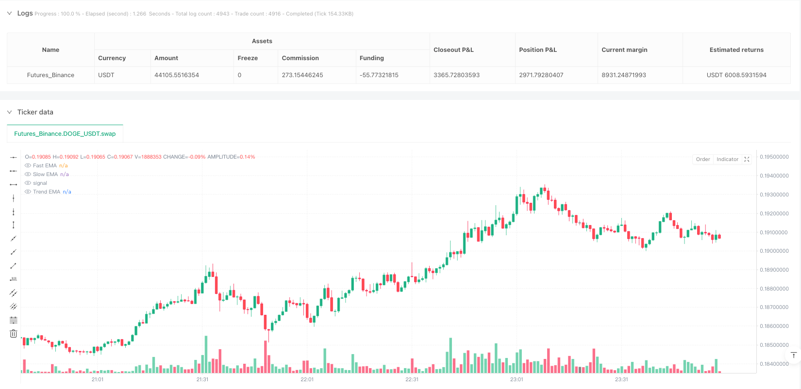
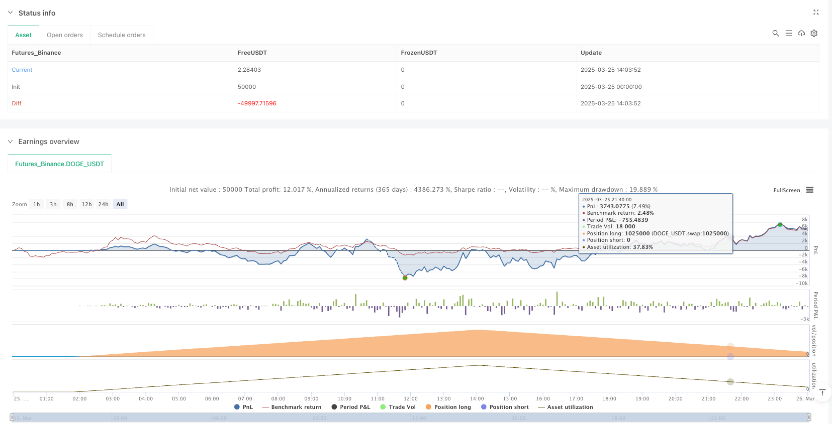
[trans]

概述

多周期波动跟踪量化策略是一种基于价格波动区间的交易系统，该策略通过计算月度、周度和日度时间周期的价格波动范围，建立动态支撑和阻力水平，进而识别潜在的交易机会。该策略核心思想是基于历史波动率计算出的价格区间，利用多周期分析方法进行交叉验证，在价格突破特定波动区间时产生交易信号。该系统特别关注周线和月线级别的支撑阻力水平，通过这些关键价格点位的交互作用，识别出高概率的入场和出场点位。

策略原理

该策略的基本原理建立在价格波动区间和多周期分析的基础上。具体来说，策略通过以下方式工作：

1. 多周期数据获取：策略首先通过request.security函数获取月度(M)、周度(W)和日度(D)三个时间周期的价格数据，包括收盘价、最高价和最低价。

2. 动态波动区间计算：利用获取的价格数据，策略计算出多个基于波动率的价格水平：

   • 上方波动区域：使用公式(((高点-低点)*(1.1/系数))+(收盘价))，其中系数分别为2和4，对应不同距离的阻力位。
   • 下方波动区域：使用公式((收盘价)-((高点-低点)*(1.1/系数)))，计算不同距离的支撑位。
   • 系数为2时产生的区域(H4/L4)表示更远的价格区域，系数为4时产生的区域(H3/L3)表示更靠近当前价格的区域。

3. 入场逻辑：

   • 多头入场条件：当前K线的前一根K线收盘价高于开盘价(上涨K线)，并且收盘价突破了周线和月线的关键支撑位(LW3和LMN3)以及周线阻力位(HW3)。
   • 这种复合条件表明价格不仅突破了短期波动区间，还获得了更高时间周期的确认。

4. 出场逻辑：

   • 空头入场(实际是多头仓位的出场)条件：价格开盘低于周线区域的支撑和阻力位(LW3和HW3)。
   • 获利了结条件(profitsave变量)：策略还定义了一个获利了结条件，当出现反转K线且反转力度较大(下跌幅度超过前一天上涨幅度)，并且开盘价和收盘价都位于周线阻力位上方时触发。

5. 图形展示：策略将关键的支撑阻力位绘制在图表上，主要显示月线和周线的H3和L3水平，使用不同颜色进行区分，方便交易者可视化分析。此外，当触发获利了结信号时，图表会显示相应的箭头标记。

策略优势

1. 多周期协同分析：通过整合月线、周线和日线数据，策略能够捕捉到不同时间周期的市场结构，增强信号的可靠性。与单一时间周期策略相比，多周期分析能够更全面地把握市场趋势。

2. 基于波动率的适应性：策略使用的支撑阻力位是基于历史价格波动计算的，而非固定数值，这使得策略能够自动适应不同市场环境和波动率变化。

3. 明确的风险管理框架：通过设定基于波动率的出场条件，策略为交易者提供了相对客观的止损和获利了结机制，有助于控制单笔交易风险。

4. 趋势确认机制：策略要求价格不仅要突破支撑位，还需要上涨K线形态，这种组合条件有助于过滤虚假突破信号。

5. 视觉直观：通过在图表上绘制关键价格水平和信号标记，交易者可以直观理解市场结构和潜在交易机会，便于实时决策和策略调整。

策略风险

1. 滞后性风险：策略使用前一周期的数据计算支撑阻力位，在快速波动的市场中，这种滞后性可能导致错过最佳入场点或过早出场。

2. 假突破风险：即使设有多重确认条件，市场仍可能出现假突破，特别是在低流动性或高波动性市场环境中。解决方法包括增加交易量确认，或设定更严格的突破条件。

3. 参数敏感性：策略使用的系数(1.1/2和1.1/4)对结果影响较大，不同市场和时期可能需要不同的优化参数。建议进行充分的历史回测和参数优化。

4. 相关性风险：代码中包含对BTCUSD的参考(虽然在最终条件中被注释掉)，这表明策略可能考虑了资产间相关性。如果市场相关性发生变化，策略性能可能受到影响。

5. 缺乏完整的止损机制：虽然策略定义了出场条件，但没有明确的基于价格的止损设置，这可能导致在极端市场条件下面临过大损失。建议添加固定止损或基于ATR的动态止损机制。

策略优化方向

1. 完善风险管理：添加明确的止损机制，例如基于ATR(平均真实范围)的动态止损，或设定最大亏损百分比。同时，可以引入分批获利机制，在不同价格水平分阶段减仓。

2. 参数自适应：目前策略使用固定的波动率系数(1.1/2和1.1/4)，可以考虑让这些参数根据市场波动性自动调整。例如，在高波动期可使用更大的系数，低波动期使用更小的系数。

3. 增加过滤器：引入趋势强度指标(如ADX)或波动率指标(如ATR)作为附加过滤条件，只在趋势明确或波动性合适的环境中交易，避免在盘整或过度波动的市场中频繁交易。

4. 时间过滤：添加时间过滤机制，避开重大经济数据发布或低流动性时段的交易，提高信号质量。

5. 整合量能分析：价格突破需要足够的交易量支持才具有持续性，建议在策略中添加交易量确认条件，例如要求突破时的交易量高于前几个周期的平均值。

6. 优化系统参数：通过深入的历史回测和步进分析，找出不同市场环境下的最优参数组合，甚至可以考虑开发动态参数调整机制。

总结

多周期波动跟踪量化策略是一个基于价格波动区间的交易系统，通过整合多个时间周期的价格数据，计算动态支撑阻力水平，识别高概率的交易机会。该策略最大的特点是利用不同时间周期的协同作用，通过交叉验证提高交易信号的可靠性。

策略的核心优势在于其适应性和多周期分析框架，使其能够在不同市场环境中保持有效性。然而，使用者需要注意策略存在的滞后性、假突破风险和参数敏感性等问题，并通过完善的风险管理措施来控制潜在损失。

通过对策略的持续优化，特别是在风险管理、参数自适应和过滤机制方面的改进，该策略有潜力成为一个稳健的交易系统。最重要的是，交易者应该理解策略背后的逻辑，而不仅仅是机械地执行信号，这样才能在市场条件变化时做出适当的调整。 ||

Overview

The Multi-Timeframe Volatility Tracking Quantitative Strategy is a trading system based on price volatility ranges. This strategy establishes dynamic support and resistance levels by calculating price fluctuation ranges across monthly, weekly, and daily timeframes to identify potential trading opportunities. The core concept revolves around price zones calculated from historical volatility, using multi-timeframe analysis for cross-validation, and generating trading signals when price breaks through specific volatility zones. The system particularly focuses on weekly and monthly support and resistance levels, identifying high-probability entry and exit points through the interaction of these key price levels.

Strategy Principles

The strategy is built on the foundation of price volatility ranges and multi-timeframe analysis. Specifically, it works as follows:

1. Multi-Timeframe Data Acquisition: The strategy first obtains price data for monthly (M), weekly (W), and daily (D) timeframes using the request.security function, including closing prices, highs, and lows.

2. Dynamic Volatility Range Calculation: Using the acquired price data, the strategy calculates multiple volatility-based price levels:

   • Upper volatility zones: Using the formula (((high-low)*(1.1/factor))+(close)), where factors of 2 and 4 correspond to resistance levels at different distances.
   • Lower volatility zones: Using the formula ((close)-((high-low)*(1.1/factor))) to calculate support levels at varying distances.
   • Zones produced with a factor of 2 (H4/L4) represent more distant price areas, while zones with a factor of 4 (H3/L3) represent areas closer to the current price.

3. Entry Logic:

   • Long entry condition: The previous candle closed higher than its open (bullish candle), and the closing price broke through both weekly and monthly key support levels (LW3 and LMN3) as well as the weekly resistance level (HW3).
   • This compound condition indicates that the price not only broke through the short-term volatility range but also received confirmation from higher timeframes.

4. Exit Logic:

   • Short entry condition (effectively an exit for long positions): Price opens below the weekly support and resistance levels (LW3 and HW3).
   • Profit-taking condition (profitsave variable): The strategy also defines a profit-taking condition triggered when a reversal candle appears with significant reversal strength (downward movement exceeding the previous day's upward movement), and both the opening and closing prices are above the weekly resistance level.

5. Graphical Display: The strategy plots key support and resistance levels on the chart, primarily displaying monthly and weekly H3 and L3 levels, using different colors for distinction to facilitate visual analysis by traders. Additionally, when profit-taking signals are triggered, arrow markers appear on the chart.

Strategy Advantages

1. Multi-Timeframe Synergistic Analysis: By integrating monthly, weekly, and daily data, the strategy can capture market structures across different timeframes, enhancing signal reliability. Compared to single-timeframe strategies, multi-timeframe analysis provides a more comprehensive grasp of market trends.

2. Volatility-Based Adaptability: The support and resistance levels used by the strategy are calculated based on historical price volatility rather than fixed values, allowing the strategy to automatically adapt to different market environments and volatility changes.

3. Clear Risk Management Framework: By setting volatility-based exit conditions, the strategy provides traders with relatively objective stop-loss and profit-taking mechanisms, helping to control risk in individual trades.

4. Trend Confirmation Mechanism: The strategy requires not only price breakouts but also bullish candle patterns, which helps filter out false breakout signals.

5. Visual Intuitiveness: By plotting key price levels and signal markers on the chart, traders can intuitively understand market structure and potential trading opportunities, facilitating real-time decision-making and strategy adjustments.

Strategy Risks

1. Lag Risk: The strategy uses data from previous periods to calculate support and resistance levels, which in rapidly fluctuating markets may lead to missing optimal entry points or exiting too early.

2. False Breakout Risk: Even with multiple confirmation conditions, false breakouts may still occur, especially in low-liquidity or high-volatility market environments. Solutions include adding volume confirmation or setting stricter breakout conditions.

3. Parameter Sensitivity: The coefficients used by the strategy (1.1/2 and 1.1/4) significantly impact results, and different markets and periods may require different optimized parameters. Thorough historical backtesting and parameter optimization are recommended.

4. Correlation Risk: The code includes references to BTCUSD (although commented out in the final conditions), suggesting the strategy may consider inter-asset correlations. If market correlations change, strategy performance may be affected.

5. Lack of Complete Stop-Loss Mechanism: Although the strategy defines exit conditions, there is no explicit price-based stop-loss setting, which could lead to excessive losses in extreme market conditions. Adding fixed stop-losses or ATR-based dynamic stop-losses is recommended.

Strategy Optimization Directions

1. Improve Risk Management: Add explicit stop-loss mechanisms, such as ATR-based dynamic stop-losses or maximum loss percentage settings. Additionally, consider implementing a staged profit-taking mechanism to partially reduce positions at different price levels.

2. Parameter Self-Adaptation: The strategy currently uses fixed volatility coefficients (1.1/2 and 1.1/4). Consider allowing these parameters to adjust automatically based on market volatility. For example, use larger coefficients during high-volatility periods and smaller coefficients during low-volatility periods.

3. Add Filters: Introduce trend strength indicators (such as ADX) or volatility indicators (such as ATR) as additional filtering conditions, trading only in environments with clear trends or appropriate volatility, avoiding frequent trading in ranging or excessively volatile markets.

4. Time Filtering: Add time filtering mechanisms to avoid trading during major economic data releases or low-liquidity periods, improving signal quality.

5. Integrate Volume Analysis: Price breakouts need sufficient trading volume to be sustainable. Consider adding volume confirmation conditions to the strategy, such as requiring breakout volume to be higher than the average of previous periods.

6. Optimize System Parameters: Through in-depth historical backtesting and walk-forward analysis, identify optimal parameter combinations for different market environments, and even consider developing a dynamic parameter adjustment mechanism.

Summary

The Multi-Timeframe Volatility Tracking Quantitative Strategy is a trading system based on price volatility ranges that identifies high-probability trading opportunities by integrating price data across multiple timeframes and calculating dynamic support and resistance levels. The strategy's most distinctive feature is its utilization of synergies between different timeframes, improving trading signal reliability through cross-validation.

The core advantages of the strategy lie in its adaptability and multi-timeframe analytical framework, enabling it to maintain effectiveness across various market environments. However, users need to be aware of issues such as lag, false breakout risks, and parameter sensitivity, and implement comprehensive risk management measures to control potential losses.

Through continuous optimization of the strategy, particularly improvements in risk management, parameter self-adaptation, and filtering mechanisms, this strategy has the potential to become a robust trading system. Most importantly, traders should understand the logic behind the strategy rather than merely executing signals mechanically, enabling appropriate adjustments when market conditions change.[/trans]

Source (PineScript)

/*backtest
start: 2025-03-25 00:00:00
end: 2025-03-26 00:00:00
period: 1m
basePeriod: 1m
exchanges: [{"eid":"Futures_Binance","currency":"DOGE_USDT"}]
*/

//@version=6
strategy("DOGE/USDT 5X Scalping Strategy", overlay=true, margin_long=20, margin_short=0)

// === Core Parameters ===
fastEMA = input.int(3, "Fast EMA Length", minval=1, maxval=20)
slowEMA = input.int(8, "Slow EMA Length", minval=2, maxval=50) 
trendEMA = input.int(55, "Trend EMA Length", minval=10, maxval=200)
atrPeriod = input.int(14, "ATR Period", minval=1, maxval=50)
tradeInterval = input.int(72, "Minutes Between Trades", minval=1, maxval=1440)

// Risk Management
slMultiplier = input.float(1.2, "Stop-Loss (ATR Multiple)", minval=0.5, maxval=5.0, step=0.1)
tpMultiplier = input.float(2.0, "Take-Profit (ATR Multiple)", minval=0.5, maxval=10.0, step=0.1)
riskPct = input.float(1.0, "Risk Per Trade (%)", minval=0.1, maxval=10.0, step=0.1)
leverage = 5.0  // Fixed 5x leverage

// === Calculate Indicators ===
fastLine = ta.ema(close, fastEMA)
slowLine = ta.ema(close, slowEMA)
trendLine = ta.ema(close, trendEMA)
atrValue = ta.atr(atrPeriod)

// === Visualize Indicators ===
// Using explicit colors to ensure visibility
fastColor = #2196F3  // Blue
slowColor = #FF9800  // Orange
trendColor = #757575  // Gray

p1 = plot(fastLine, "Fast EMA", color=fastColor, linewidth=2)
p2 = plot(slowLine, "Slow EMA", color=slowColor, linewidth=2)
p3 = plot(trendLine, "Trend EMA", color=trendColor, linewidth=1)

// Cross detection for visualization
crossUp = ta.crossover(fastLine, slowLine)
crossDown = ta.crossunder(fastLine, slowLine)
plotshape(crossUp, "EMA Cross Up", style=shape.triangleup, location=location.belowbar, color=color.green, size=size.small)
plotshape(crossDown, "EMA Cross Down", style=shape.triangledown, location=location.abovebar, color=color.red, size=size.small)

// === Trade Logic ===
// Cooldown mechanism
var int lastTradeBarIndex = 0
timeElapsed = (bar_index - lastTradeBarIndex) >= tradeInterval
noActivePosition = strategy.position_size == 0

// Entry conditions
emaCross = ta.crossover(fastLine, slowLine)
trendFilter = close > trendLine
validEntry = emaCross and trendFilter and timeElapsed and noActivePosition

// Position sizing calculation
equity = strategy.equity
riskAmount = equity * (riskPct / 100)
stopDistance = atrValue * slMultiplier
positionSize = math.round((riskAmount / stopDistance) * leverage) // Round to whole tokens for DOGE

// Visualize entry signals
plotshape(validEntry, "Entry Signal", style=shape.circle, location=location.belowbar, color=color.lime, size=size.normal)

// === Strategy Execution ===
if (validEntry)
    // Entry
    strategy.entry("Long", strategy.long, qty=positionSize)
    
    // Set exit points
    stopPrice = close - (atrValue * slMultiplier)
    targetPrice = close + (atrValue * tpMultiplier)
    strategy.exit("Exit", "Long", stop=stopPrice, limit=targetPrice)
    
    // Reset cooldown timer
    lastTradeBarIndex := bar_index
    

Detail

https://www.fmz.com/strategy/489149

Last Modified

2025-04-02 10:50:32