246 lines
14 KiB
Markdown
246 lines
14 KiB
Markdown

|
|
|||
|
|
> Name
|
|||
|
|
|
|||
|
|
多重斐波那契优化时间入场策略-Multi-Fibonacci-Optimal-Time-Entry-Strategy
|
|||
|
|
|
|||
|
|
> Author
|
|||
|
|
|
|||
|
|
ianzeng123
|
|||
|
|
|
|||
|
|
> Strategy Description
|
|||
|
|
|
|||
|
|
|
|||
|
|
|
|||
|
|
|
|||
|
|
|
|||
|
|
[trans]
|
|||
|
|
|
|||
|
|
#### 概述
|
|||
|
|
|
|||
|
|
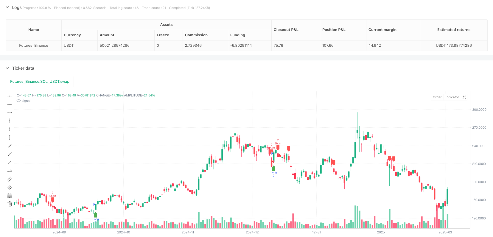
多重斐波那契优化时间入场策略是一种基于市场结构和价格回调水平的量化交易系统,该策略融合了ICT(内部市场理论)的OTE(优化时间入场)概念与传统的斐波那契回调分析。策略核心是通过识别市场的关键摇摆高点和低点,计算多个斐波那契回调水平,并在价格与特定斐波那契水平(0.705)交叉且同时满足其他条件时生成交易信号。这种方法旨在捕捉价格在重要支撑阻力位的反弹或突破,从而在趋势延续中获取优势入场点。
|
|||
|
|
|
|||
|
|
#### 策略原理
|
|||
|
|
|
|||
|
|
策略的工作原理可以分为几个关键步骤:
|
|||
|
|
|
|||
|
|
1. **摇摆点识别**:策略首先使用指定长度(默认20个周期)来识别市场中的摇摆高点和低点。这些点被定义为在给定周期内的最高价和最低价。
|
|||
|
|
|
|||
|
|
2. **斐波那契回调计算**:一旦确定了摇摆高点和低点,策略计算六个关键的斐波那契回调水平:0.272、0.382、0.5、0.618、0.705和0.786。这些水平是基于摇摆高低点之间的价格区间计算得出。
|
|||
|
|
|
|||
|
|
3. **视觉辅助**:策略在图表上绘制出这些斐波那契水平,每个水平使用不同颜色以便于区分。这为交易者提供了视觉参考,帮助识别关键的价格区域。
|
|||
|
|
|
|||
|
|
4. **入场条件**:
|
|||
|
|
- 多头入场:当价格向上穿越0.705斐波那契水平,且收盘价高于0.618水平时触发。
|
|||
|
|
- 空头入场:当价格向下穿越0.705斐波那契水平,且收盘价低于0.618水平时触发。
|
|||
|
|
|
|||
|
|
这种入场逻辑结合了价格突破(穿越0.705水平)和趋势确认(相对于0.618水平的位置)两个条件,旨在减少虚假信号并增强策略稳健性。
|
|||
|
|
|
|||
|
|
#### 策略优势
|
|||
|
|
|
|||
|
|
多重斐波那契优化时间入场策略具有几个显著优势:
|
|||
|
|
|
|||
|
|
1. **精确的入场点**:通过结合斐波那契回调水平和价格交叉条件,策略能够提供精确的入场信号,减少了盲目入场的风险。
|
|||
|
|
|
|||
|
|
2. **视觉清晰**:策略在图表上直观显示所有关键的斐波那契水平,使交易者能够清晰理解市场结构和潜在的支撑阻力区域。
|
|||
|
|
|
|||
|
|
3. **灵活适应性**:策略允许调整摇摆长度参数,使其能够适应不同的市场条件和时间周期。
|
|||
|
|
|
|||
|
|
4. **双向交易**:策略同时支持多头和空头交易,能够在不同市场环境中捕捉机会。
|
|||
|
|
|
|||
|
|
5. **减少噪音**:通过使用0.705和0.618两个关键水平的组合条件,策略有效过滤了市场噪音,减少了虚假突破的可能性。
|
|||
|
|
|
|||
|
|
6. **基于市场结构**:策略基于真实的市场结构(摇摆高低点)计算入场区域,而不是使用任意或固定的价格水平。
|
|||
|
|
|
|||
|
|
#### 策略风险
|
|||
|
|
|
|||
|
|
尽管该策略具有优势,但也存在一些潜在风险:
|
|||
|
|
|
|||
|
|
1. **参数敏感性**:摇摆长度参数的选择对策略性能有显著影响。较短的长度可能导致过度交易,而较长的长度可能导致错过重要机会。
|
|||
|
|
|
|||
|
|
2. **市场环境依赖**:在高波动或横盘整理市场中,策略可能产生较多虚假信号。策略在趋势明确的市场中表现最佳。
|
|||
|
|
|
|||
|
|
3. **回撤风险**:尽管使用多个条件筛选信号,但市场仍可能在入场后出现显著回撤,尤其是在重大新闻或事件影响时。
|
|||
|
|
|
|||
|
|
4. **不包含止损机制**:当前策略代码未定义止损水平,这增加了资金管理风险。
|
|||
|
|
|
|||
|
|
5. **过度依赖技术指标**:策略完全基于技术分析,忽略了基本面因素和市场情绪,这可能在某些市场环境中导致不理想结果。
|
|||
|
|
|
|||
|
|
风险缓解措施可以包括:添加明确的止损规则、结合其他技术指标进行确认、在重大经济事件前暂停交易,以及根据不同市场条件动态调整参数。
|
|||
|
|
|
|||
|
|
#### 策略优化方向
|
|||
|
|
|
|||
|
|
该策略有几个可能的优化方向:
|
|||
|
|
|
|||
|
|
1. **动态止损/止盈**:实现基于ATR或斐波那契水平的动态止损和止盈机制,以保护利润并限制损失。
|
|||
|
|
|
|||
|
|
2. **多时间周期确认**:添加更高时间周期的趋势确认条件,以确保交易方向与更大趋势一致。
|
|||
|
|
|
|||
|
|
3. **交易量过滤器**:在入场条件中加入交易量确认,以增加价格突破的可靠性。
|
|||
|
|
|
|||
|
|
4. **动态参数调整**:实现基于市场波动性自动调整摇摆长度参数的机制,使策略能够更好地适应不同市场环境。
|
|||
|
|
|
|||
|
|
5. **加入市场情绪指标**:结合RSI、MACD或随机指标等额外的技术指标,提供更多的交易确认。
|
|||
|
|
|
|||
|
|
6. **入场优化**:实现分批入场策略,在价格达到特定斐波那契水平时分多次建立头寸,以降低入场时机的风险。
|
|||
|
|
|
|||
|
|
7. **历史模式识别**:添加识别历史上成功模式的逻辑,当当前市场条件与过去成功交易模式相似时增加仓位大小。
|
|||
|
|
|
|||
|
|
这些优化可以显著提高策略的稳健性、盈利能力和风险调整后的回报。特别是添加止损机制和多时间周期确认可能是最紧急和最有价值的改进。
|
|||
|
|
|
|||
|
|
#### 总结
|
|||
|
|
|
|||
|
|
多重斐波那契优化时间入场策略是一个结合了ICT理论和斐波那契回调分析的精细量化交易系统。通过识别关键的市场结构和价格交互,策略能够提供精确的入场信号,适用于多种市场环境。其核心优势在于精确的入场机制和清晰的视觉反馈,但需要注意市场环境变化和资金管理风险。
|
|||
|
|
|
|||
|
|
通过实施建议的优化措施,尤其是添加止损机制、多时间周期确认和动态参数调整,该策略有潜力成为一个全面且稳健的交易系统。最终,该策略为交易者提供了一个结构化的框架,用于识别和利用市场中的优化入场机会。 ||
|
|||
|
|
|
|||
|
|
#### Overview
|
|||
|
|
|
|||
|
|
The Multi-Fibonacci Optimal Time Entry Strategy is a quantitative trading system based on market structure and price retracement levels, integrating ICT (Inner Circle Trader) OTE (Optimal Time Entry) concepts with traditional Fibonacci retracement analysis. The core of the strategy is to identify key market swing highs and lows, calculate multiple Fibonacci retracement levels, and generate trading signals when price crosses a specific Fibonacci level (0.705) while simultaneously meeting other conditions. This approach aims to capture price rebounds or breakouts at significant support and resistance levels, thereby gaining advantageous entry points during trend continuation.
|
|||
|
|
|
|||
|
|
#### Strategy Principles
|
|||
|
|
|
|||
|
|
The strategy's working principles can be divided into several key steps:
|
|||
|
|
|
|||
|
|
1. **Swing Point Identification**: The strategy first uses a specified length (default 20 periods) to identify swing highs and lows in the market. These points are defined as the highest and lowest prices within the given period.
|
|||
|
|
|
|||
|
|
2. **Fibonacci Retracement Calculation**: Once swing highs and lows are determined, the strategy calculates six key Fibonacci retracement levels: 0.272, 0.382, 0.5, 0.618, 0.705, and 0.786. These levels are derived from the price range between the swing high and low points.
|
|||
|
|
|
|||
|
|
3. **Visual Assistance**: The strategy draws these Fibonacci levels on the chart, using different colors for each level for easy differentiation. This provides traders with visual references to help identify key price areas.
|
|||
|
|
|
|||
|
|
4. **Entry Conditions**:
|
|||
|
|
- Long entry: Triggered when price crosses above the 0.705 Fibonacci level and the closing price is higher than the 0.618 level.
|
|||
|
|
- Short entry: Triggered when price crosses below the 0.705 Fibonacci level and the closing price is lower than the 0.618 level.
|
|||
|
|
|
|||
|
|
This entry logic combines price breakout (crossing the 0.705 level) and trend confirmation (position relative to the 0.618 level) conditions, aiming to reduce false signals and enhance strategy robustness.
|
|||
|
|
|
|||
|
|
#### Strategy Advantages
|
|||
|
|
|
|||
|
|
The Multi-Fibonacci Optimal Time Entry Strategy has several notable advantages:
|
|||
|
|
|
|||
|
|
1. **Precise Entry Points**: By combining Fibonacci retracement levels and price crossing conditions, the strategy can provide precise entry signals, reducing the risk of blind entries.
|
|||
|
|
|
|||
|
|
2. **Visual Clarity**: The strategy visually displays all key Fibonacci levels on the chart, allowing traders to clearly understand market structure and potential support/resistance areas.
|
|||
|
|
|
|||
|
|
3. **Flexible Adaptability**: The strategy allows adjustment of the swing length parameter, making it adaptable to different market conditions and timeframes.
|
|||
|
|
|
|||
|
|
4. **Bidirectional Trading**: The strategy supports both long and short trades, capable of capturing opportunities in different market environments.
|
|||
|
|
|
|||
|
|
5. **Noise Reduction**: By using the combination of 0.705 and 0.618 key levels as conditions, the strategy effectively filters market noise, reducing the possibility of false breakouts.
|
|||
|
|
|
|||
|
|
6. **Market Structure Based**: The strategy calculates entry zones based on actual market structure (swing highs and lows) rather than using arbitrary or fixed price levels.
|
|||
|
|
|
|||
|
|
#### Strategy Risks
|
|||
|
|
|
|||
|
|
Despite its advantages, the strategy also presents some potential risks:
|
|||
|
|
|
|||
|
|
1. **Parameter Sensitivity**: The choice of swing length parameter has a significant impact on strategy performance. Shorter lengths may lead to overtrading, while longer lengths may cause missed opportunities.
|
|||
|
|
|
|||
|
|
2. **Market Environment Dependency**: In highly volatile or ranging markets, the strategy may produce more false signals. The strategy performs best in markets with clear trends.
|
|||
|
|
|
|||
|
|
3. **Drawdown Risk**: Despite using multiple conditions to filter signals, the market may still experience significant drawdowns after entry, especially during major news or events.
|
|||
|
|
|
|||
|
|
4. **Lack of Stop-Loss Mechanism**: The current strategy code does not define stop-loss levels, which increases money management risk.
|
|||
|
|
|
|||
|
|
5. **Over-reliance on Technical Indicators**: The strategy is entirely based on technical analysis, ignoring fundamental factors and market sentiment, which may lead to undesirable results in certain market environments.
|
|||
|
|
|
|||
|
|
Risk mitigation measures can include: adding explicit stop-loss rules, incorporating other technical indicators for confirmation, pausing trading before major economic events, and dynamically adjusting parameters based on different market conditions.
|
|||
|
|
|
|||
|
|
#### Strategy Optimization Directions
|
|||
|
|
|
|||
|
|
There are several possible optimization directions for this strategy:
|
|||
|
|
|
|||
|
|
1. **Dynamic Stop-Loss/Take-Profit**: Implement dynamic stop-loss and take-profit mechanisms based on ATR or Fibonacci levels to protect profits and limit losses.
|
|||
|
|
|
|||
|
|
2. **Multiple Timeframe Confirmation**: Add trend confirmation conditions from higher timeframes to ensure trade direction aligns with the larger trend.
|
|||
|
|
|
|||
|
|
3. **Volume Filter**: Include volume confirmation in entry conditions to increase the reliability of price breakouts.
|
|||
|
|
|
|||
|
|
4. **Dynamic Parameter Adjustment**: Implement a mechanism to automatically adjust the swing length parameter based on market volatility, allowing the strategy to better adapt to different market environments.
|
|||
|
|
|
|||
|
|
5. **Adding Market Sentiment Indicators**: Incorporate additional technical indicators such as RSI, MACD, or Stochastic to provide more trade confirmations.
|
|||
|
|
|
|||
|
|
6. **Entry Optimization**: Implement a scaling-in strategy, building positions in multiple entries as price reaches specific Fibonacci levels to reduce entry timing risk.
|
|||
|
|
|
|||
|
|
7. **Historical Pattern Recognition**: Add logic to identify historically successful patterns and increase position size when current market conditions resemble past successful trades.
|
|||
|
|
|
|||
|
|
These optimizations can significantly improve the strategy's robustness, profitability, and risk-adjusted returns. In particular, adding stop-loss mechanisms and multiple timeframe confirmation may be the most urgent and valuable improvements.
|
|||
|
|
|
|||
|
|
#### Summary
|
|||
|
|
|
|||
|
|
The Multi-Fibonacci Optimal Time Entry Strategy is a sophisticated quantitative trading system that combines ICT theory with Fibonacci retracement analysis. By identifying key market structures and price interactions, the strategy can provide precise entry signals applicable to various market environments. Its core advantages lie in its precise entry mechanism and clear visual feedback, but attention must be paid to changes in market environment and money management risks.
|
|||
|
|
|
|||
|
|
By implementing the suggested optimization measures, especially adding stop-loss mechanisms, multiple timeframe confirmation, and dynamic parameter adjustment, the strategy has the potential to become a comprehensive and robust trading system. Ultimately, this strategy provides traders with a structured framework for identifying and capitalizing on optimal entry opportunities in the market.[/trans]
|
|||
|
|
|
|||
|
|
|
|||
|
|
|
|||
|
|
> Source (PineScript)
|
|||
|
|
|
|||
|
|
``` pinescript
|
|||
|
|
/*backtest
|
|||
|
|
start: 2024-03-05 00:00:00
|
|||
|
|
end: 2025-03-03 08:00:00
|
|||
|
|
period: 1d
|
|||
|
|
basePeriod: 1d
|
|||
|
|
exchanges: [{"eid":"Futures_Binance","currency":"SOL_USDT"}]
|
|||
|
|
*/
|
|||
|
|
|
|||
|
|
//@version=6
|
|||
|
|
strategy("ICT OTE Strategy", overlay=true, default_qty_type=strategy.percent_of_equity, default_qty_value=1)
|
|||
|
|
|
|||
|
|
// Input settings
|
|||
|
|
length = input.int(20, title="Swing Length")
|
|||
|
|
showFibs = input.bool(true, title="Show Fibonacci Levels")
|
|||
|
|
|
|||
|
|
find_swing_high(len) =>
|
|||
|
|
ta.highest(high, len) == high
|
|||
|
|
|
|||
|
|
find_swing_low(len) =>
|
|||
|
|
ta.lowest(low, len) == low
|
|||
|
|
|
|||
|
|
// Identify swing high and low
|
|||
|
|
var float swingHigh = na
|
|||
|
|
var float swingLow = na
|
|||
|
|
|
|||
|
|
if find_swing_high(length)
|
|||
|
|
swingHigh := high
|
|||
|
|
|
|||
|
|
if find_swing_low(length)
|
|||
|
|
swingLow := low
|
|||
|
|
|
|||
|
|
// Define Fibonacci retracement levels
|
|||
|
|
fibLow = swingLow
|
|||
|
|
fibHigh = swingHigh
|
|||
|
|
|
|||
|
|
fib_level(start, end, level) =>
|
|||
|
|
start - (start - end) * level
|
|||
|
|
|
|||
|
|
fib_0_705 = fib_level(fibHigh, fibLow, 0.705)
|
|||
|
|
fib_0_786 = fib_level(fibHigh, fibLow, 0.786)
|
|||
|
|
fib_0_618 = fib_level(fibHigh, fibLow, 0.618)
|
|||
|
|
fib_0_5 = fib_level(fibHigh, fibLow, 0.5)
|
|||
|
|
fib_0_382 = fib_level(fibHigh, fibLow, 0.382)
|
|||
|
|
fib_0_272 = fib_level(fibHigh, fibLow, 0.272)
|
|||
|
|
|
|||
|
|
// Entry conditions based on OTE
|
|||
|
|
longEntry = ta.crossover(close, fib_0_705) and close > fib_0_618
|
|||
|
|
shortEntry = ta.crossunder(close, fib_0_705) and close < fib_0_618
|
|||
|
|
|
|||
|
|
// Strategy execution
|
|||
|
|
if longEntry
|
|||
|
|
strategy.entry("Long", strategy.long)
|
|||
|
|
if shortEntry
|
|||
|
|
strategy.entry("Short", strategy.short)
|
|||
|
|
|
|||
|
|
plotshape(series=longEntry, location=location.belowbar, color=color.green, style=shape.labelup, title="Long Entry")
|
|||
|
|
plotshape(series=shortEntry, location=location.abovebar, color=color.red, style=shape.labeldown, title="Short Entry")
|
|||
|
|
|
|||
|
|
```
|
|||
|
|
|
|||
|
|
> Detail
|
|||
|
|
|
|||
|
|
https://www.fmz.com/strategy/484912
|
|||
|
|
|
|||
|
|
> Last Modified
|
|||
|
|
|
|||
|
|
2025-03-05 09:45:25
|