strategies/多指标突破与反转交易策略结合开盘价区间优化的双重进场系统-Multi-Indicator-Breakout-and-Reversal-Trading-Strategy-A-Dual-Entry-System-with-Opening-Range-Optimization.md

> Name

多指标突破与反转交易策略结合开盘价区间优化的双重进场系统-Multi-Indicator-Breakout-and-Reversal-Trading-Strategy-A-Dual-Entry-System-with-Opening-Range-Optimization

> Author

ianzeng123

> Strategy Description

![IMG](https://www.fmz.com/upload/asset/2d88d1b2e8ee5b207afbc.png)
![IMG](https://www.fmz.com/upload/asset/2d89f0e2c199949a912db.png)


[trans]

## 概述

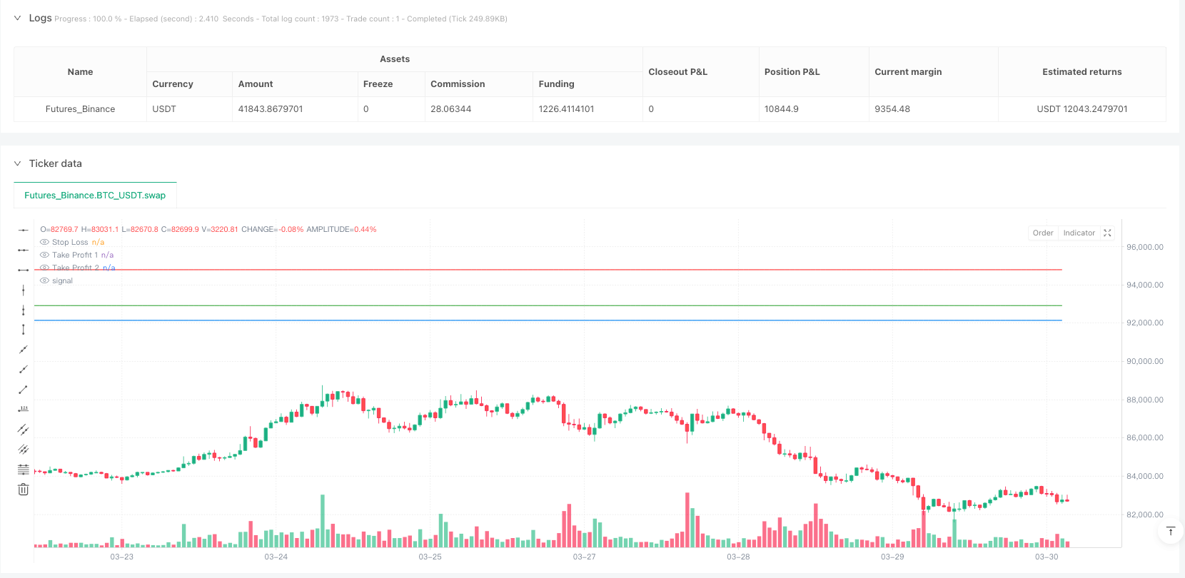
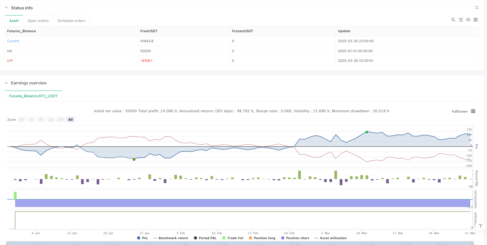
多指标突破与反转交易策略是一种结合技术分析指标与价格行为的量化交易方法，旨在捕捉市场中的两类主要交易机会：价格反转和趋势突破。该策略巧妙地整合了移动平均线、相对强弱指数(RSI)、平均真实范围(ATR)和交易量加权平均价格(VWAP)等多种技术指标，同时引入开盘区间突破(ORB)机制以增强入场信号的可靠性。策略采用双目标止盈设计，并具备自动将止损调整至盈亏平衡点的风险管理机制，特别适合在短时间周期（如2分钟图表）上应用，通过参数调整也可适用于更高的时间周期。

## 策略原理

该策略的核心原理是通过多重指标过滤和确认，识别三类潜在有利的交易机会：

1. **反转交易信号**：
   - 多头反转：当价格上穿50期简单移动平均线(SMA50)，RSI低于超卖阈值(默认30)，且价格低于VWAP，同时总体趋势向上(价格高于SMA200)时触发。
   - 空头反转：当价格下穿SMA50，RSI高于超买阈值(默认70)，且价格高于VWAP，同时总体趋势向下(价格低于SMA200)时触发。

2. **趋势突破信号**：
   - 多头突破：当9期指数移动平均线(EMA9)上穿20期指数移动平均线(EMA20)，价格高于VWAP，且总体趋势向上时触发。
   - 空头突破：当EMA9下穿EMA20，价格低于VWAP，且总体趋势向下时触发。

3. **开盘区间突破(ORB)信号**：
   - 多头ORB：当价格突破开盘前特定数量柱(默认15柱)形成的最高价，且交易量超过开盘区间平均交易量的预设倍数(默认1.5倍)时触发。
   - 空头ORB：当价格跌破开盘前形成的最低价，且交易量满足阈值条件时触发。

策略使用ATR指标计算动态止损位置，通过回溯特定周期(默认7)的最低价/最高价并加减ATR值的倍数(默认0.5)来设定。入场后，策略设置两个止盈目标：
- 第一目标(TP1)：风险的0.5倍(默认)，平仓25%的头寸
- 第二目标(TP2)：风险的1.1倍(默认)，平仓剩余75%的头寸

当第一个止盈目标达成后，策略自动将止损调整至入场价格(盈亏平衡点)，有效保护已获得的利润。

## 策略优势

1. **多样化的入场信号**：通过整合反转、突破和开盘区间突破三种不同的入场信号，策略能够适应多种市场环境，有效增加交易机会，同时保持较高的信号质量。

2. **完善的风险管理**：策略采用分级止盈机制，允许部分获利同时保留潜在的更大收益。当达到第一个止盈目标时，自动将止损调整至盈亏平衡点，实现"让利润奔跑"的同时保护资本。

3. **动态止损计算**：使用ATR指标计算止损位置，使止损水平能够根据市场波动性动态调整，更准确地反映当前市场状况，避免过于紧密或过于宽松的止损设置。

4. **交易量确认**：特别在ORB信号中引入交易量确认机制，要求突破时的交易量必须超过开盘区间平均交易量的特定倍数，有效过滤低质量突破。

5. **趋势过滤**：通过200期简单移动平均线(SMA200)判断长期趋势方向，确保交易方向与主要趋势一致，提高交易成功率。

6. **资金管理整合**：策略内置资金管理机制，限制每个交易使用的资金比例(默认50%的资本)，确保资金多元化配置，降低单一交易的风险敞口。

## 策略风险

1. **指标滞后性**：策略主要依赖移动平均线等滞后指标，可能导致在快速变化的市场中入场时机延迟，错过较佳入场点或导致不必要的损失。

   解决方法：考虑增加前瞻性指标如价格行为模式识别，或缩短较长周期移动平均线的参数，提高对市场变化的敏感性。

2. **参数敏感性**：大量可调参数(如EMA长度、RSI阈值、ATR系数等)使策略优化变得复杂，且可能导致过度拟合历史数据而在未来市场中表现不佳。

   解决方法：采用适当的参数优化方法，如前向验证、蒙特卡洛模拟，避免过度优化；或者使用固定参数，专注于更加稳健的规则设计。

3. **多信号冲突**：在某些市场环境下，不同的入场信号可能产生相互矛盾的交易建议，导致策略表现不稳定。

   解决方法：建立更严格的信号优先级系统，或引入额外的确认机制，确保只在高概率情况下执行交易。

4. **止损跳空风险**：在波动较大或流动性较低的市场中，价格可能跳空越过止损位置，导致实际损失超过预期。

   解决方法：考虑使用期权对冲策略，或在高波动性市场条件下增加止损距离，甚至临时降低头寸规模。

5. **系统性风险敞口**：策略同时运行多个相关交易，可能在市场剧烈波动时面临系统性风险，导致多个交易同时亏损。

   解决方法：实施全局风险控制，限制总体头寸规模，或在不同资产类别间分散交易，降低相关性风险。

## 策略优化方向

1. **引入机器学习模型**：将机器学习算法应用于指标权重优化或市场环境分类，可自动调整不同市场条件下各指标的相对重要性，提高策略的适应性。

   优化理由：传统的固定权重指标组合难以适应不同市场阶段，而机器学习可以从历史数据中自动学习最优的指标组合模式。

2. **整合市场情绪指标**：加入波动率指数(VIX)或高频市场情绪指标，帮助策略更好地识别市场环境，调整入场条件和风险参数。

   优化理由：市场情绪对短期价格走势有显著影响，整合这类指标可以提前捕捉市场转折点，优化入场和出场时机。

3. **动态调整止盈比例**：基于历史波动性或支撑阻力水平自动调整止盈目标，使策略在不同波动环境中都能获取合理的利润。

   优化理由：固定的风险回报比在不同市场环境中可能不够灵活，动态调整可以在高波动市场中设置更远的目标，低波动市场中设置更保守的目标。

4. **引入时间过滤器**：加入基于市场时段的过滤机制，避免在低波动或不利时段交易，如市场开盘后的前几分钟或流动性较低的午间时段。

   优化理由：市场活动在一天中不同时段表现出明显差异，时间过滤可以帮助策略专注于最具优势的交易时段。

5. **优化头寸规模计算**：从固定资金比例转为基于波动性的头寸规模计算，在高波动时期自动减小头寸，低波动时期适当增加头寸。

   优化理由：风险与市场波动性直接相关，动态头寸管理可以保持更一致的风险水平，改善长期风险调整后收益。

## 总结

多指标突破与反转交易策略是一个融合多种技术分析方法的综合性量化交易系统，通过整合反转、趋势突破和开盘区间突破信号，结合完善的风险管理和资金管理机制，旨在捕捉各种市场环境下的交易机会。策略的核心优势在于信号多元化、风险控制完善以及参数可定制性强，特别适合短周期交易。同时，策略也面临指标滞后性、参数敏感性和信号冲突等潜在风险，需要通过引入机器学习、市场情绪分析、动态止盈设置等方向进行进一步优化。总体而言，这是一个设计全面、思路清晰的交易策略框架，为量化交易者提供了良好的起点，通过持续改进和适当的风险管理，有潜力成为一个稳健可靠的交易系统。|| 

## Overview

The Multi-Indicator Breakout and Reversal Trading Strategy is a quantitative trading approach that combines technical analysis indicators with price action to capture two primary trading opportunities in the market: price reversals and trend breakouts. This strategy cleverly integrates multiple technical indicators including moving averages, Relative Strength Index (RSI), Average True Range (ATR), and Volume Weighted Average Price (VWAP), while also incorporating an Opening Range Breakout (ORB) mechanism to enhance entry signal reliability. The strategy employs a dual target profit-taking design and features an automatic risk management mechanism that adjusts the stop loss to breakeven, making it particularly suitable for short timeframes (such as 2-minute charts), with parameter adjustments allowing for application to higher timeframes as well.

## Strategy Principles

The core principle of this strategy is to identify three potential favorable trading opportunities through multiple indicator filtering and confirmation:

1. **Reversal Trading Signals**:
   - Long Reversal: Triggered when price crosses above the 50-period Simple Moving Average (SMA50), RSI is below the oversold threshold (default 30), price is below VWAP, and the overall trend is up (price above SMA200).
   - Short Reversal: Triggered when price crosses below SMA50, RSI is above the overbought threshold (default 70), price is above VWAP, and the overall trend is down (price below SMA200).

2. **Trend Breakout Signals**:
   - Long Breakout: Triggered when the 9-period Exponential Moving Average (EMA9) crosses above the 20-period Exponential Moving Average (EMA20), price is above VWAP, and the overall trend is up.
   - Short Breakout: Triggered when EMA9 crosses below EMA20, price is below VWAP, and the overall trend is down.

3. **Opening Range Breakout (ORB) Signals**:
   - Long ORB: Triggered when price breaks above the highest price formed during a specific number of bars (default 15) at the opening, and volume exceeds a preset multiple (default 1.5x) of the average volume in the opening range.
   - Short ORB: Triggered when price breaks below the lowest price formed at the opening, and volume meets the threshold condition.

The strategy uses the ATR indicator to calculate dynamic stop loss positions by looking back at the lowest/highest price over a specific period (default 7) and adding/subtracting a multiple (default 0.5) of the ATR value. After entry, the strategy sets two profit targets:
- First target (TP1): 0.5 times the risk (default), closing 25% of the position
- Second target (TP2): 1.1 times the risk (default), closing the remaining 75% of the position

When the first profit target is achieved, the strategy automatically adjusts the stop loss to the entry price (breakeven point), effectively protecting the profit already gained.

## Strategy Advantages

1. **Diversified Entry Signals**: By integrating three different entry signals—reversal, breakout, and opening range breakout—the strategy can adapt to various market environments, effectively increasing trading opportunities while maintaining high signal quality.

2. **Comprehensive Risk Management**: The strategy adopts a tiered profit-taking mechanism, allowing partial profit realization while retaining potential for greater returns. When the first profit target is reached, the stop loss is automatically adjusted to breakeven, achieving "let profits run" while protecting capital.

3. **Dynamic Stop Loss Calculation**: Using the ATR indicator to calculate stop loss positions allows the stop level to dynamically adjust based on market volatility, more accurately reflecting current market conditions and avoiding overly tight or loose stop loss settings.

4. **Volume Confirmation**: A volume confirmation mechanism is introduced especially in ORB signals, requiring that breakout volume must exceed a specific multiple of the average volume in the opening range, effectively filtering low-quality breakouts.

5. **Trend Filtering**: Using the 200-period Simple Moving Average (SMA200) to determine long-term trend direction ensures that trading direction is consistent with the main trend, improving the success rate of trades.

6. **Integrated Capital Management**: The strategy has built-in capital management mechanisms, limiting the proportion of funds used for each trade (default 50% of capital), ensuring diversified capital allocation and reducing risk exposure from any single trade.

## Strategy Risks

1. **Indicator Lag**: The strategy primarily relies on lagging indicators such as moving averages, which may lead to delayed entry timing in rapidly changing markets, missing optimal entry points or causing unnecessary losses.

   Solution: Consider adding forward-looking indicators such as price action pattern recognition, or shortening the parameters of longer-period moving averages to increase sensitivity to market changes.

2. **Parameter Sensitivity**: Numerous adjustable parameters (such as EMA length, RSI threshold, ATR coefficient, etc.) make strategy optimization complex and may lead to overfitting historical data, resulting in poor performance in future markets.

   Solution: Adopt appropriate parameter optimization methods, such as forward validation or Monte Carlo simulation, to avoid over-optimization; or use fixed parameters and focus on more robust rule design.

3. **Multi-Signal Conflicts**: In certain market environments, different entry signals may produce contradictory trading recommendations, leading to unstable strategy performance.

   Solution: Establish a stricter signal priority system or introduce additional confirmation mechanisms to ensure trades are executed only in high-probability situations.

4. **Stop Loss Gap Risk**: In volatile or less liquid markets, prices may gap beyond stop loss positions, resulting in actual losses exceeding expectations.

   Solution: Consider using options hedging strategies, or increase stop loss distance in high-volatility market conditions, or even temporarily reduce position size.

5. **Systemic Risk Exposure**: Running multiple related trades simultaneously, the strategy may face systemic risk during severe market volatility, leading to multiple trades losing at the same time.

   Solution: Implement global risk control, limit overall position size, or diversify trades across different asset classes to reduce correlation risk.

## Strategy Optimization Directions

1. **Introduce Machine Learning Models**: Applying machine learning algorithms to indicator weight optimization or market environment classification can automatically adjust the relative importance of various indicators under different market conditions, improving strategy adaptability.

   Optimization Rationale: Traditional fixed-weight indicator combinations struggle to adapt to different market phases, while machine learning can automatically learn the optimal indicator combination patterns from historical data.

2. **Integrate Market Sentiment Indicators**: Adding volatility indices (VIX) or high-frequency market sentiment indicators helps the strategy better identify market environments and adjust entry conditions and risk parameters.

   Optimization Rationale: Market sentiment significantly influences short-term price movements; integrating such indicators can capture market turning points in advance, optimizing entry and exit timing.

3. **Dynamically Adjust Profit-Taking Ratios**: Automatically adjusting profit targets based on historical volatility or support/resistance levels allows the strategy to capture reasonable profits in different volatility environments.

   Optimization Rationale: Fixed risk-reward ratios may not be flexible enough in different market environments; dynamic adjustment can set more distant targets in high-volatility markets and more conservative targets in low-volatility markets.

4. **Introduce Time Filters**: Adding filtering mechanisms based on market sessions helps avoid trading during low-volatility or unfavorable periods, such as the first few minutes after market opening or low-liquidity noon sessions.

   Optimization Rationale: Market activity shows significant differences across different periods of the day; time filtering can help the strategy focus on the most advantageous trading sessions.

5. **Optimize Position Size Calculation**: Switching from fixed capital percentage to volatility-based position sizing, automatically reducing positions during high-volatility periods and appropriately increasing positions during low-volatility periods.

   Optimization Rationale: Risk is directly related to market volatility; dynamic position management can maintain more consistent risk levels, improving long-term risk-adjusted returns.

## Summary

The Multi-Indicator Breakout and Reversal Trading Strategy is a comprehensive quantitative trading system that integrates various technical analysis methods. By combining reversal, trend breakout, and opening range breakout signals with comprehensive risk and capital management mechanisms, it aims to capture trading opportunities across various market environments. The core advantages of the strategy lie in signal diversification, robust risk control, and strong parameter customizability, making it particularly suitable for short-term trading. Meanwhile, the strategy also faces potential risks such as indicator lag, parameter sensitivity, and signal conflicts, requiring further optimization through machine learning integration, market sentiment analysis, dynamic profit-taking settings, and other approaches. Overall, this is a comprehensively designed, clearly structured trading strategy framework that provides quantitative traders with a solid starting point. Through continuous improvement and appropriate risk management, it has the potential to become a robust and reliable trading system.[/trans]



> Source (PineScript)

``` pinescript
/*backtest
start: 2025-01-01 00:00:00
end: 2025-03-31 00:00:00
period: 1h
basePeriod: 1h
exchanges: [{"eid":"Futures_Binance","currency":"BTC_USDT"}]
*/

//@version=5
strategy("Reversal & Breakout Strategy with ORB", overlay=true, pyramiding=2, initial_capital=50000)

// --- Inputs ---
ema9Length = input.int(9, "9 EMA Length", minval=1)
ema20Length = input.int(20, "20 EMA Length", minval=1)
sma50Length = input.int(50, "50 SMA Length", minval=1)
sma200Length = input.int(200, "200 SMA Length", minval=1)
rsiLength = input.int(14, "RSI Length", minval=1)
rsiOverbought = input.int(70, "RSI Overbought", minval=0, maxval=100)
rsiOversold = input.int(30, "RSI Oversold", minval=0, maxval=100)
atrLength = input.int(14, "ATR Length", minval=1)
stopMulti = input.float(0.5, "Stop Loss ATR Multiplier", minval=0.1, step=0.1)
stopLookback = input.int(7, "Stop Loss Lookback", minval=1)
rr1 = input.float(0.5, "Risk:Reward Target 1", minval=0.1, step=0.1)
rr2 = input.float(1.1, "Risk:Reward Target 2", minval=0.1, step=0.1)
target1Percent = input.float(25, "Profit % Target 1", minval=0, maxval=100)
orbBars = input.int(15, "Opening Range Bars", minval=1, tooltip="Number of bars to define the opening range (e.g., 15 bars = 30 min on 2-min chart)")
volThreshold = input.float(1.5, "Volume Threshold Multiplier", minval=1.0, step=0.1, tooltip="Volume must be this multiple of the opening range average")

// --- Indicators ---
// Moving Averages
ema9 = ta.ema(close, ema9Length)
ema20 = ta.ema(close, ema20Length)
sma50 = ta.sma(close, sma50Length)
sma200 = ta.sma(close, sma200Length)

// VWAP
vwapValue = ta.vwap(close)

// RSI
rsi = ta.rsi(close, rsiLength)

// ATR
atr = ta.atr(atrLength)

// --- Opening Range Breakout ---
var float openingRangeHigh = na
var float openingRangeLow = na
var float openingRangeAvgVol = na
if bar_index < orbBars
    openingRangeHigh := na
    openingRangeLow := na
    openingRangeAvgVol := na
else if bar_index == orbBars
    openingRangeHigh := ta.highest(high, orbBars)
    openingRangeLow := ta.lowest(low, orbBars)
    openingRangeAvgVol := ta.sma(volume, orbBars)

orbLong = not na(openingRangeHigh) and ta.crossover(close, openingRangeHigh) and volume > openingRangeAvgVol * volThreshold
orbShort = not na(openingRangeLow) and ta.crossunder(close, openingRangeLow) and volume > openingRangeAvgVol * volThreshold

// --- Trend Detection ---
trendUp = close > sma200
trendDown = close < sma200

// --- Reversal Conditions ---
reversalLong = ta.crossover(close, sma50) and rsi < rsiOversold and close < vwapValue and trendUp
reversalShort = ta.crossunder(close, sma50) and rsi > rsiOverbought and close > vwapValue and trendDown

// --- Range Breakout Conditions ---
breakoutLong = ta.crossover(ema9, ema20) and close > vwapValue and trendUp
breakoutShort = ta.crossunder(ema9, ema20) and close < vwapValue and trendDown

// Combine conditions
longCondition = (reversalLong or breakoutLong or orbLong)
shortCondition = (reversalShort or breakoutShort or orbShort)

// --- Calculate Position Size ---
equityPerPosition = 25000.0  // $50,000 / 2 positions
positionSizeLong = math.floor(equityPerPosition / close)
positionSizeShort = math.floor(equityPerPosition / close)

// --- Stop Loss Calculation ---
longStop = ta.lowest(low, stopLookback) - (atr * stopMulti)
shortStop = ta.highest(high, stopLookback) + (atr * stopMulti)

// --- Variables to Store Trade Levels ---
var float tradeStop = na
var float tradeTarget1 = na
var float tradeTarget2 = na
var float initialPositionSize = na
var bool breakEvenSet = false  // Track if stop has been moved to break-even
var float stopLevel = na       // Dedicated variable for stop loss in exits
var float target1Level = na    // Dedicated variable for first take profit
var float target2Level = na    // Dedicated variable for second take profit
var float qtyTotal = na        // Track total quantity

// --- Reset Levels Before New Trade ---
var bool newTrade = false
if longCondition or shortCondition
    newTrade := true
else
    newTrade := false

if strategy.position_size == 0 and newTrade
    tradeStop := na
    tradeTarget1 := na
    tradeTarget2 := na
    stopLevel := na
    target1Level := na
    target2Level := na
    initialPositionSize := na
    qtyTotal := na
    breakEvenSet := false

// --- Strategy Entries ---
if longCondition and strategy.position_size == 0
    strategy.entry("Long", strategy.long, qty=positionSizeLong * 2)
    tradeStop := longStop
    stopLevel := longStop
    stopDistance = close - tradeStop
    tradeTarget1 := close + (stopDistance * rr1)
    tradeTarget2 := close + (stopDistance * rr2)
    target1Level := tradeTarget1
    target2Level := tradeTarget2
    initialPositionSize := positionSizeLong * 2
    qtyTotal := positionSizeLong * 2
    breakEvenSet := false  // Reset break-even flag

if shortCondition and strategy.position_size == 0
    strategy.entry("Short", strategy.short, qty=positionSizeShort * 2)
    tradeStop := shortStop
    stopLevel := shortStop
    stopDistance = tradeStop - close
    tradeTarget1 := close - (stopDistance * rr1)
    tradeTarget2 := close - (stopDistance * rr2)
    target1Level := tradeTarget1
    target2Level := tradeTarget2
    initialPositionSize := positionSizeShort * 2
    qtyTotal := positionSizeShort * 2
    breakEvenSet := false  // Reset break-even flag

// --- Trade Exits ---
if strategy.position_size > 0
    qty_tp1 = qtyTotal * (target1Percent / 100)
    qty_tp2 = qtyTotal * ((100 - target1Percent) / 100)
    strategy.exit("Long Exit 1", "Long", qty=qty_tp1, stop=stopLevel, limit=target1Level)
    strategy.exit("Long Exit 2", "Long", qty=qty_tp2, stop=stopLevel, limit=target2Level)

if strategy.position_size < 0
    qty_tp1 = qtyTotal * (target1Percent / 100)
    qty_tp2 = qtyTotal * ((100 - target1Percent) / 100)
    strategy.exit("Short Exit 1", "Short", qty=qty_tp1, stop=stopLevel, limit=target1Level)
    strategy.exit("Short Exit 2", "Short", qty=qty_tp2, stop=stopLevel, limit=target2Level)

// --- Move Stop to Break-even ---
if strategy.position_size != 0 and not na(initialPositionSize) and not breakEvenSet
    if math.abs(strategy.position_size) < math.abs(initialPositionSize)
        tradeStop := strategy.position_avg_price
        stopLevel := strategy.position_avg_price
        tradeTarget1 := na  // Clear first target for plotting
        breakEvenSet := true  // Mark break-even as set

// --- Manual Close Fallback ---
if strategy.position_size > 0
    if close >= target2Level or close <= stopLevel
        strategy.close("Long", qty=qtyTotal, comment="Manual Close")

if strategy.position_size < 0
    if close <= target2Level or close >= stopLevel
        strategy.close("Short", qty=qtyTotal, comment="Manual Close")

// --- Reset Levels When No Position ---
if strategy.position_size == 0 and not newTrade
    tradeStop := na
    tradeTarget1 := na
    tradeTarget2 := na
    stopLevel := na
    target1Level := na
    target2Level := na
    initialPositionSize := na
    qtyTotal := na
    breakEvenSet := false

// --- Plotting ---
plot(tradeStop, title="Stop Loss", color=color.red, linewidth=1, style=plot.style_linebr)
plot(tradeTarget1, title="Take Profit 1", color=color.green, linewidth=1, style=plot.style_linebr)
plot(tradeTarget2, title="Take Profit 2", color=color.blue, linewidth=1, style=plot.style_linebr)
```

> Detail

https://www.fmz.com/strategy/489048

> Last Modified

2025-04-01 16:00:37